

If you are reading this from the safe little life you inhabit, you are already desensitized to the US-Iran ceasefire peek-a-boo. If you accuse me of callousness to compare violence to a children’s game I’ll blame it on out-of-sight, out-of-mind distance and the limits of attention. But callousness is often just that as opposed to intentional venom so guilty-as-charged. Throw your stones.
There is (I think) minority view that the rhetorical whiplash has a profit motive. There’s the taco-flavored version which favors peace not for any strategic or humanitarian reason but because asset prices prefer it. This is the populist interpretation, if the everyman it hopes to appease is the retired boomer who’s overweight stocks because Trump’s a good businessman and will make shares rise.
There’s also the less egalitarian profit motive in that timing ceasefire game-on and game-off news coincides with less liquid and more easily manipulable oil futures markets. The news that Trump has made $1.4B in income from crypto, while BTC has been halved, doesn’t inspire a ton of confidence in the White House compliance department. (Of course, that news is not really information insofar as information is defined as a surprise or material Bayesian update to a prior.)
This pattern or at least its vibe is almost a meme on twitter. Of course, when I want to dig up tweets from sensible accounts recounting the moves I can’t remember them and Grok only surfaces bot-quality examples:

Whether there is manipulation or not is a matter for the CFTC (which is now a dictatorship, by the way, so don’t hold your breath on discovery), but the pattern is real. Recall this outstanding interview with Onyx, the world’s largest oil market maker, founder Greg Newman:
The oil market historically has been quite orderly around its market hours. But after 7:30pm our time — which is the US close, up to maybe 6pm their time — that window is meant to be dead. It’s meant to not really trade, and it’s been very, very active around these times. So now we’re doing the hours later on, to see what’s going on, because the order book will reveal things. If you’ve got the visibility of all the contracts, that’s where you’re in the best position to know: has someone selected something in particular, and what could that mean? Because there’s no other reason why you would trade at that time. If you want to hedge, you go for the peak times. If you want to speculate, you want liquidity, so again you go for peak times. So why are you trading in these evening-to-nighttime trades? It makes no sense, other than maybe you’ve just got the information. And I think Trump knows that as well, because he makes a lot of his announcements either on the weekend — when the market will gap up or down — or at night. And we’re forced to be very ready up until the actual close of the exchange now, rather than the close of the market day.
This is where my interests turn predictably dorky.
What does this mean for pricing oil options?
Thanks for asking.
It brings us to a familiar topic for long-time readers:
variance time
I’m not going to re-hash all the theory. For review you can watch this:
If you want more detail, you can read these:
- Understanding Variance Time — translating between 252-day vs 365-day models and the idea of dirty vs clean vols.
- The Dirties Are Down, the Cleans Are Up — cleaning implied vol of the calendar’s day-count artifacts
- Weekend Theta — how a weekend actually decays, and how wall time and voltime diverge strongest when the market is closed
- Pricing 0DTEs — the same clock questions at the daily / intraday scale.
In this post, we:
- see how the overnight and weekend’s share of asset price volatility has changed by looking at data across liquid ETFs. The oil pattern jumps off the page, it is not just vibes.
- explain how these effects bias the IV artifacts (ie the changes in IV that come from the imperfect day count in your chosen model)
- suggest what this means for pricing 0dte
- give you a web-based notebook so you can choose your own dates and tickers to compute what the overnights and weekends have been “worth”
Partitioning variance
Perhaps the most common way to compute realized volatility is to annualize a sample of daily logreturns. This is known as “close-to-close” volatility.
It’s imperfect or in nerd parlance takes a long time to “converge” on an accurate estimate of an asset’s true volatility. This is easy to see if we consider the case where an asset closes at the same price each day but experiences a 5% intraday range. C-to-C vol is poorly represents the risk when it says this asset is zero vol. The market would “correct” this by happily bidding 40% vol for the straddle.
At moontower.ai we use a blend of:
- Close-to-Close
- Parkinson
- Hodges-Tompkins
- Yang-Zhang
I’m in the Euan Sinclair camp on this topic — there’s no special sauce realized-vol calc that distinguishes measures but these other methods are cheap, effective improvements that include more data via daily price ranges.
💡 Many types of estimators try to forecast realized volatility based on past data. If that interests you, the NYU Stern Volatility Lab documentation is a great start.
Conveniently, “close” is not the only standard market data field. We can separate the overnight return from the daily return by using the “open” price. I call this partitioning variance. You are invited and encouraged to adapt this concept beyond the scope of this post.
Method
For each day, take two log returns:
- the overnight gap,
r_co = ln(open / prior close) - full day,
r_cc = ln(close / prior close).
rco = ln(open / prior close) rcc = ln(close / prior close)
While we normally speak of volatility because it’s interpretable as a standard deviation, it’s simpler to not deal with the square roots and just compute variances.
💡The real reason we prefer variance is many important option metrics (p/l’s, straddle prices) scale linearly with respect to variance but are power functions in volatility.
Under a zero-drift assumption (harmless when dealing with daily data), variance is just the mean of squared returns. We can compute the overnight variance ratio over a trailing window:
overnight variance ratio = Σ rco² / Σ rcc²
We will do this for a 63-day window (about a quarter of a year’s worth of returns).
If the price was unchanged from the close to the open everyday the ratio would be zero. The market doesn’t usually open at the previous day’s close so the ratio is between 0 and 1. Just as a matter of connecting dots, this also means that the BSM assumption that prices are continuous is obviously wrong.
If the ratio is .50 that says 1/2 the variance in the 24-hour move occurred overnight.
Let’s look at SPY and USO (ETF holding prompt WTI oil futures) to track this rolling ~3 month metric for the past decade.
Implementation
Data: yfinance daily OHLC (auto-adjusted for splits & dividends);
Window: 63-day rolling; zero-drift (no mean subtraction)
Lookback: 6/30/16 — 6/30/26
You can run versions with your own tickers and parameters here:
Results
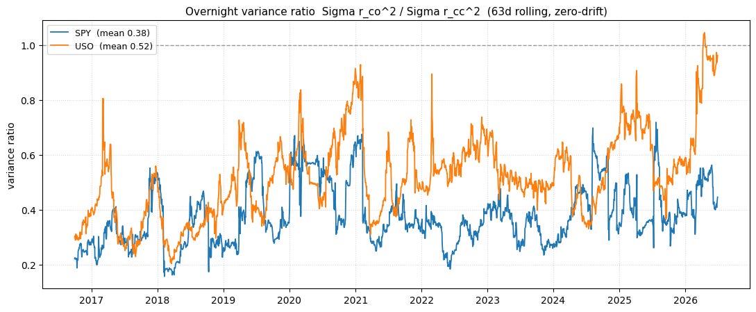
SPY averages 0.38 while USO averages 0.52.
But in 2026, USO ran near 0.82!
Even with a full-quarter window’s smoothing, oil’s overnight variance ratio poked above 1.0 in mid-April 2026, the most overnight-dominated stretch of the entire decade including COVID and the invasion of Ukraine. Oil’s overnight variance actually matched its full-day variance.
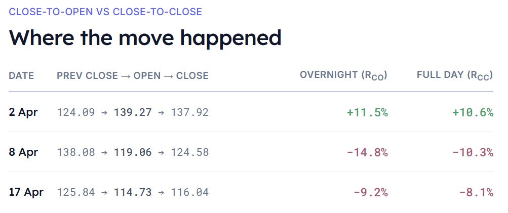
The combination of these overnight gaps moves clustering in a 2-week period and the emphasis that squaring returns puts on the sums was pushed the entire window’s ratio towards 1.0.
But what does this mean for option pricing?
The variance-time architecture
Understanding Variance Time explains how an option model’s year-length is a choice that influences how implied vol changes as time passes. But that IV change is not necessarily reflecting any change in consensus volatility. It is purely an artifact of how we define t in Black-Scholes.
Two common models bracket that choice:
- The 252-day (trading-day) model takes the extreme view that weekends and holidays carry zero variance-time.
- The 365-day (calendar) model takes the opposite extreme — a Saturday is worth exactly as much as a Tuesday.
If there is structurally less volatility in a market that is closed (for example weekends and holidays) then the market then embedding that in how t unfolds makes changes in IV more meaningful and less of an artifact. We care about IV because its changes are supposed to reflect the market’s assessment of risk. If it’s confounded by a ruler that assumes variance time and wall-time are the same, we muddy the meaning of IV changes.
[Weekend Theta explains why VIX is observed to rise on Mondays. It’s a measurement artifact that goes away if you treat Saturday and Sunday as a fraction of a typical trading day.]
The weekend variance share is the dial between day-count conventions. The more variance a market infers for the weekend, the more the 365-day model is right. That makes sense. That’s a world where Saturday and Wednesday contain similar amounts of volatility.
Again for most contexts this doesn’t matter, but for anyone running a strategy that cares granularly about relative IV changes between options this is required work.
💡The python notebook I linked to allows you to compute the weekend’s share of variance as well!
0DTE and the question of what’s the straddle worth at the open?
If you believe that 50% of an asset’s variance comes from the overnight change, then the 24-hour straddle should lose half its value at the open since straddle price is proportional to variance. If you want to think in vol terms.
[Notice that this corresponds to ~70% of the volatility having transpired because of sqrt(.50). Just for scaling practice, this is the same as saying you have to cut volatility of the ATM straddle by 70% to halve its value.]
The one-night stand trade
If the straddle was overpriced after the open, the way to test or trade this would be to buy the next-day straddle at the close to capture the overnight volatility and kick her/him outta bed on when the options open!
The trade feels like you’re saying “the IV is too high” but to a model that assumes vol time passes non-linearly as opposed to clock time (intuitively you understand that the last 15 minutes of the trading day includes more volatility than say 15 minutes at lunchtime) the trade is saying “most of the day’s vol time has already passed…the options haven’t take out enough theta yet”.
A more accurate vol time schedule can allow you to consider strategies like “short USO vol on the open and buy equity vol, reverse into the close”. I do think you can kluge it by just noticing that on the same calendar USO IV falls faster during the day. But it’s a bit less direct to associate that with an infrastructure that locates that trade within the context of regimes which have a higher proportion of overnight variance which are not so much making statement about how IV changes but in how it’s distributed and concentrated around the clock.
Wrapping up
Review Pricing 0DTEs. Remember option streaming software generally allows users to specify how vol time passes relative to wall time (the regular clock). In fact, they will often allow this down to the asset level so you could have a different schedule for gold or stocks or oil. This makes sense. An asset that depends on US weather reports released during the day should have a different schedule than one that is globally traded and sensitive to politics across time zones.
Play with the collab notebook or fork the code to develop an understanding of overnight and weekend variance with respect to the trading day. This intuition gives you a baseline from which to consider how perps and 24-hour trading might influence what option markets embed (and therefore might need to unlearn!).
That should be plenty to chew on for today.
Have an awesome weekend and Happy 250 years America!