using tick data for spot-vol correlations

If spot is up 1% and vol is up 1%, what delta lean do you need?

Say you’re long 1,000 vega and vol is 40%. Vol ticks up 0.4 (1% relative move), so P&L is +$400. To stay flat, you need to lean short $400 / 1% = $40,000 of underlying.

Compactly:

delta lean = −vega × σ × β

-$400 = -1000 x 40% x 1.0

σ is the vol in percent and β is the relative or percent vol move per 1% spot move.

(Note that short vega flips the sign.)

I introduced this idea in embedding spot-vol correlation in option deltas. It’s a response to a familiar problem where your option model says you’re long $50mm of SPY but acts like it’s only long $40mm.

But where does β actually come from?

In that post, we started with correlation as a given and built an adjustment. Later we used VXX/SPY beta as a proxy for spot/vol beta.

This is adequate if you’re trading SPY against VIX futures or using the general spot-vol relationship as an input to sizing in portfolio construction.

But if you’re in the daily weeds of running a market-neutral option book, those estimates are riddled with at least 2 glaring problems:

1. They update too slowly since it’s typical to use at least daily data for both correlations and volatilities.
2. They are too low-resolution. If you have options inventory, you don’t care what “vol” is doing broadly because composite measures like VIX and floating measures like “ATM vol” capture movement along the vol curve. Insofar as there’s a skew, those are already “baked in”. Option p/l depends on changes in option premium and the portion of that you are trading, the vega, cares about changes in the strike vol.

It’s one thing to say SPX vol increases as the index falls but that is expected from the skew. The question is “do the strike vols actually increase as the index falls and with what vol beta?”

That’s the sensitivity you need to inform your lean.

I must confess, this exact topic has a small audience. The market-neutral vol book jockey is definitely the type of job you would only find in a pretty advanced economy. We’re well past pineapples for coconut barter here. If that’s you, well, you don’t need convincing to read on. Nobody talks to you as it is, but here I am bringing flowers and chocolate.

But for the sake of the wider population, I’d say the absolute specifics are not the best reason to follow along. But there are reasons.

If you are an option market maker who doesn’t get their model handed to them from on high with marching orders to trust it, you’ve had to hack together mods like you’re Xzibit in Pimp My Ride. Being both a non-quant and surviving several turns of 10,000 hours of repetition, I’ve hacked together many solutions to option pricing and modeling. They ain’t gonna win any awards, but you can sketch ‘em on a napkin. They’re useful enough to work, but juuuust dumb enough to keep you paranoid.

Let’s step through this one and see if everyone can learn a little somethin somethin.

Pulling it from the data

We want to know how strike vol changes with the spot price, not the ATM vol.

Here’s the recipe:

1. Select the nearest strike to ATM of the prior close.
2. Track that strike’s IV alongside spot through the session. Always use the OTM option on the strike. So if the spot price dips below the strike, use the call IV and vice versa.
3. Regress the interval-to-interval relative vol changes on the percent spot changes. The slope is β.

It sounds simple, but as soon as you get your hands dirty, you realize there’s lots of microdecisions you need to make if you want to distill a useful number from the sea of dots you’re about to create.

For example, you can measure every minute, but you’re destined for pathological results since you are just going to be dividing by small numbers.

You’ll find more success and little cost (hell, negative cost, since it’s less data to fetch) to widen your intervals to 5 or 15 minutes AND throwing out the intervals where spot barely moved.

Look, a 5-minute bar where SPY moved 1 basis point contains no information about how vol responds to spot, but a regression greedily gobbles a cloudy sample to report back that there’s no slope. Maybe your eyes are lyin’ to you?

Could be.

If your business is to stare at screens all day and you feel the slope, but your method of snapshotting says there is none, maybe you really are being fooled by randomness. But…maybe your measurement choices are not well-matched to the phenomenon you feel. What can I say, welcome to trading, grab a helmet. If they could hand you a manual at birth and pat your bum to “go get em”, everyone would be rich and sane.

So we hack.

Exclude any interval where the spot move is smaller than half the expected move for that interval. We’re already tracking the strike’s vol, and any used napkin on the floor in Ceres Cafe tells us that 16 vol asset moves about 1% a day. Vol isn’t uniformly distributed through the day, but we’re traders, not scientists. 78 5-minute intervals it is.

1%/√78 means 11 bps per 5 minutes. So we set a gate at half that, call it 5 bps for SPY. We’re going to do this for more names. Same logic assigns SLV a gate of 16 bps, USO gets 18 bps. So any interval where the spot doesn’t move more than the gate is ignored. Notice that the vol used is the one observed at the start of each interval from the prior day’s strike vol, so there’s no look-ahead bias on the gate size.

We are going to look at the change in strike vol vs change in spot for SPY, GLD, SLV, and USO across two two-week windows with dense intraday sampling: June 8–22 and August 3–14, 5-minute intervals throughout.

Eight ticker-fortnights. Here’s the board:

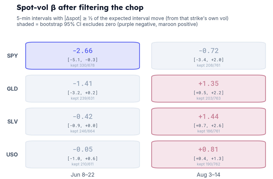
From the eight regressions, we observe a few striking stories (pun intended and without remorse).

• SPY has a significant negative spot/strike vol correlation in June but no material correlation in August.
• Every commodity has a significant positive spot/strike vol correlation in August.
• Notice the keep-counts: June keeps about half its intervals; August keeps a quarter. I won’t dive further into keep-counts, but it could be something interesting to noodle on. For any given vol, how many intervals would you expect to surpass some gate, and if you were to sort these results across a large cross-section of tick data, could it give you a faster-updating relative vol signal? Hacking around always leads to ideas. Most are just noise, but if you find something, there’s a decent chance it won’t be the kind of thing people are discussing on Twitter or SSRN.

Let’s zoom in closer.

The equity regime

SPY, June 8–22.

We find a mixed tape.

Three real down days (−1.0%, −1.2%, −1.2%), one +1.5% rally, and a lot of chop otherwise.

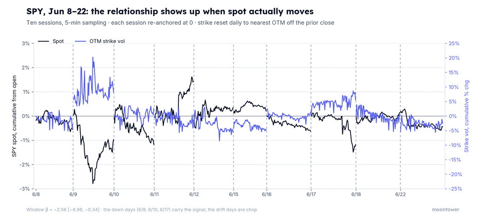
The relationship shows up when spot actually moves.

On the down days, the vol line is a rough mirror of the spot line.

In interval space:

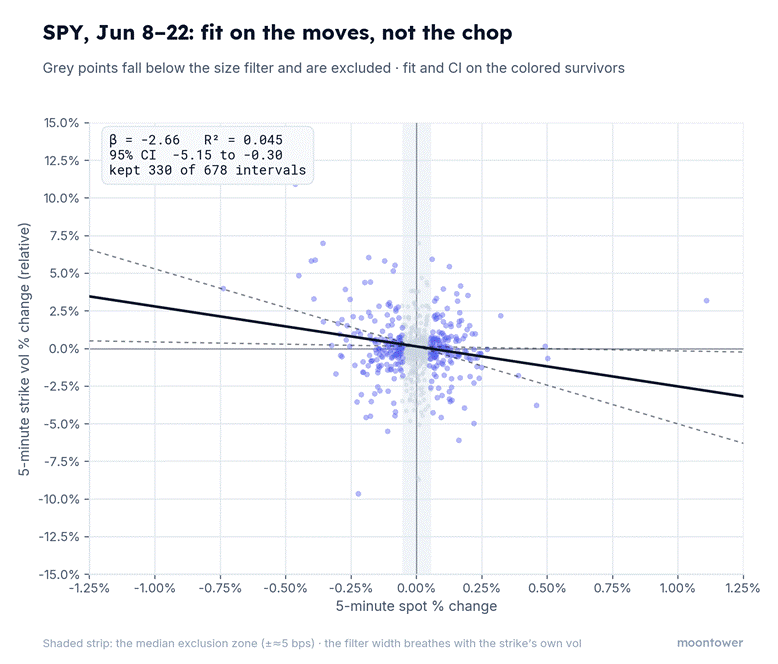
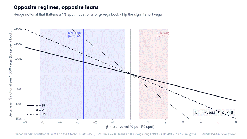
β = −2.66, bootstrap 95% CI [−5.15, −0.30] on the 330 surviving intervals.

What drives the correlation?

6/9, spot down 1%: day-β of −9.3, CI [−13.8, −3.1], R² = 0.23.

6/10, down 1.2%: −3.3, significant again.

The days that move are the days the regression works, but that’s why we want the leans anyway. They don’t matter for the chop days.

The commodity regime

Let’s look at August 3–14.

Gold was the active market that fortnight while SPY chopped around on an 11-vol doing nothing.

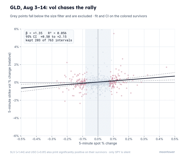
β = +1.35 [+0.50, +2.15]. Spot up, strike vol up. It’s not just movement along the vol curve.

We see the same behavior in silver, SLV printed +1.44, and to a lesser extent oil with USO β = +0.81.

Each market steepens toward its own scary side

Just as we have a concept of “up beta” and “down beta” in delta-one investing, we can split every interval by the sign of the spot move and fit β separately on each half:

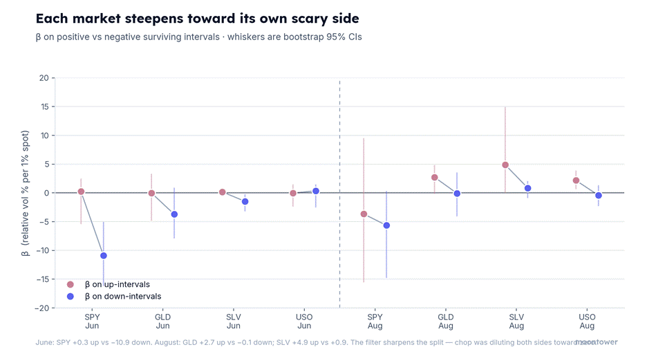
In June, the down-move slopes are steeper across the board.

In August, the commodities flip it.

GLD runs +2.7 on up-intervals against −0.1 on down, and SLV +4.9 against +0.9. The slope is steepest on the rally while equity vol lives on the break, confirming our general intuitions (comforting, right?).

But again, there are hacky things to notice.

The pooled β you fit is an average over two different states. That means a pooled estimate systematically undersizes the hedge for the scenario that motivated it. It’s profound because it means even when you dial in the right spot-strike vol beta, it will hopefully be additive on average, but it will always be precisely wrong.

Silver’s split personality

SLV, June 8–22:

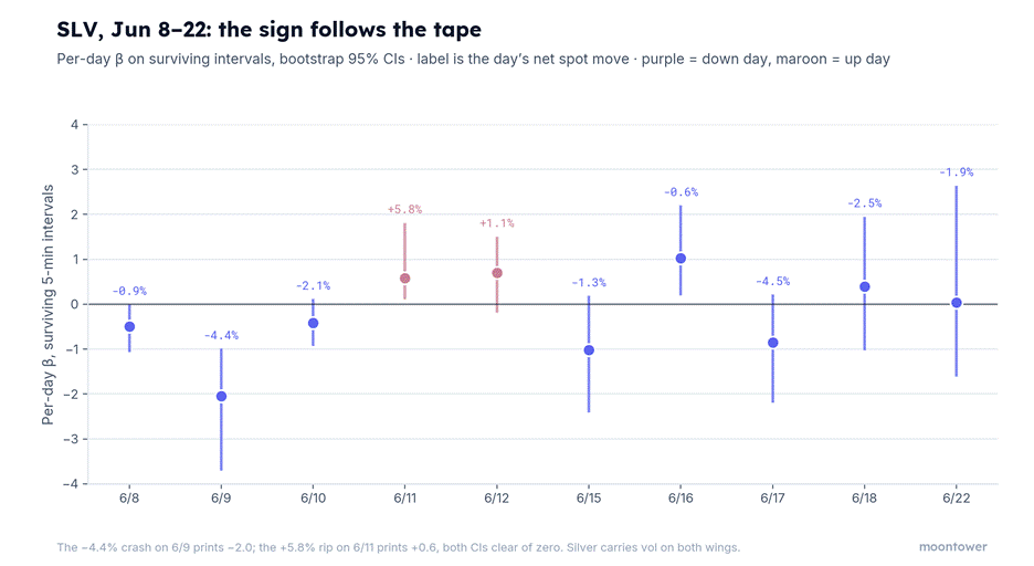
On 6/9, SLV fell 4.4% and the day-β is −2.0. Vol up as silver fell. Equity-like behavior.

On 6/11, silver ripped +5.8% and the day-β is +0.6. Vol up as silver rallied.

Nasty, because if you were short vol, the 6/9 move would encourage you to lean short delta, which only compounded your pain on 6/11.

This is going to sound counterintuitive, but this bad beat is actually an argument for why you should be handicapping spot/strike vol correlations from recent data (ie to have a quickly updating estimate rather than a conventional zoomed-out beta). The vol betas actually move around a lot at the granularity of your risk on a book with strikes in it, but you want to be calibrated to the market in front of you. That you sometimes get chopped by a flip in the spot-strike vol beta is more of an indication that vol itself needs to find a fairer level. In silver’s case, the vol was simply too low, and the market understood that regardless of the spot direction.

Duct tape all the way down

Let’s pause before using these betas to modify our positions.

I want to be clear that every specific in this post is negotiable. The half-a-sigma gate could be 0.3 or 0.6. Five-minute bars could be four or six. 5,000 resamples for the confidence intervals could be 2,000. None of it is sacred or optimized. In fact, if moving a parameter a little to the left or right dramatically changes the prescriptions, then that would be worrisome. But the solace in that is whatever you choose won’t be a fatal error. You don’t want to be Buridan’s Ass here.

Remind yourself of the problem.

1. Vol almost always shows a correlation with spot.
2. Since it’s so consistent, we should embed our vega risk into our delta lean at least for the sake of local moves. That’s all delta hedges help with in the first place anyway.
3. That correlation’s impact on our p/l is actually at the level of strike vols, not floating ATM vol, which is captured by movement along the curve. Movement along the curve has minimal impact on the vega portion of our p/l
4. We need to extract the correlation of spot to strike vol empirically
5. Strike vol to spot correlations are noisy but real. We’re going hack our way to estimating them from intraday data.

An inventory of the duct tape we collected as hackers (in parentheses, I had Claude try to identify what the formal analog might be for those inclined):

• I throw out intervals where spot barely moved, because tiny prints are mostly bid-ask wiggle and they drag the slope toward zero (errors-in-variables attenuation; the fix is a threshold estimator).
• I set that cutoff from the strike vol I’m already tracking, observed at the start of the interval so the rule can’t peek at the move it’s judging (a causal filter — measurability with respect to the information you had at the time).
• I fit up-moves and down-moves separately because the market is scared of one side more than the other (semibetas — Bollerslev, Patton and Quaedvlieg formalized splitting beta by sign).
• I get error bars by reshuffling my own data to myself 5,000 times instead of trusting a formula (the pairs bootstrap; Efron, 1979).

The benefit of hacks is they are intuitive enough to inspect and their robustness is usually self-evident. Formality is great if it works for you, but the bar for understanding is higher because the embedded assumptions in derivations can easily hide behind convenience.

The goal of this analysis is to simply be a little better at estimating the proper hedge ratio. Given that you will bother hedging, you’d rather be a little more accurate if you can. This technique helped me calibrate to the market’s most recent behavior. It’s all about collecting micro-victories on the margin of every process without ever falling into the trap of optimizing beyond the limit of what can reasonably be known. You wear your seatbelt but never confuse that for protection against a tree falling on your car.

Let’s continue.

From the regression to the lean

Time to use the betas.

You’re short 1,000 vega in SPY during that June window. Your delta is zero.

Are you flat?

Let’s use the output of the regression to establish a lean.

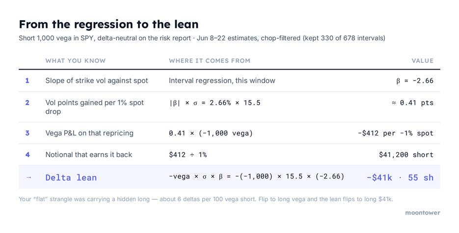
If you were long 1,000 vega, the lean flips to long $41k: your long vol position bleeds vega P&L on rallies, so you carry extra length against it.

Now run the same arithmetic on GLD in August, short 1,000 vega: β = +1.35, σ ≈ 23. Lean = −(−1,000) × 23 × 1.35 ≈ long $31,000. Opposite sign, so the short-vol gold book leans long GLD shares.

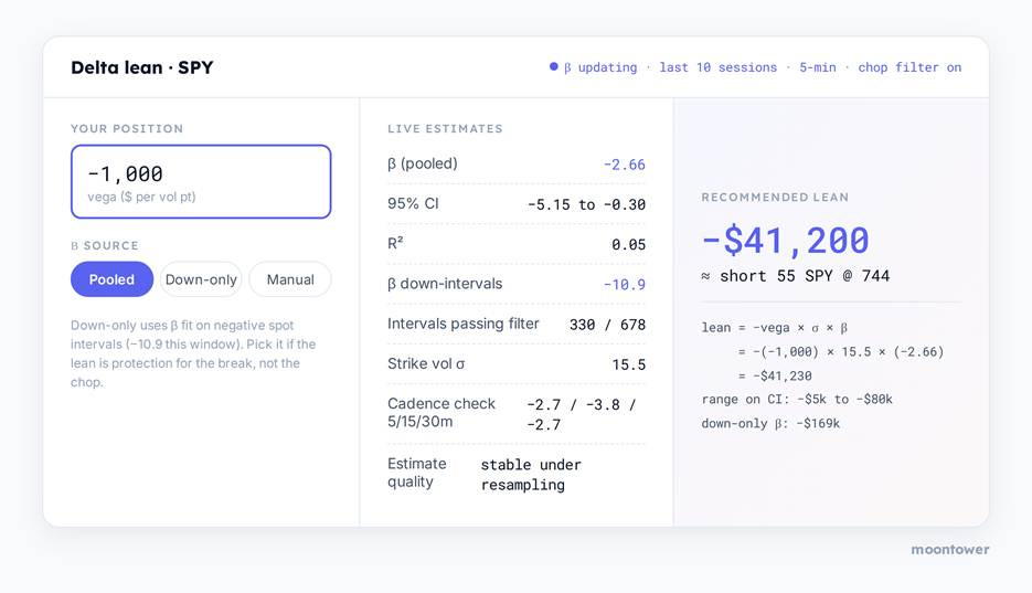
I used to keep this in a spreadsheet, but now you can just feed this post into an LLM and have a PR to give you a web-based tool:

Possible extensions

I’ve had to make decisions on all of these at some point. Again, there’s no single answer.

• Do I fit a different slope per month/expiry and apply each to the vega exposure in that month, then roll up to an aggregate lean? Or pick a single reference month, scale all my vega to it, and use that month’s empirical slope for the whole book?
• Over what range do I even trust this parameter? A slope estimated from ordinary 5-min chop is not the slope you’d want to lean on during a real shock. If the lean makes sense for small moves, does it ruin my risk slide for large moves? Remember we are embedding the behavior of vega with delta, then calling all of it delta. When push comes to shove, vega is casting a delta-shaped shadow that you can’t fully rest on.
• Reiterating the earlier questions of what sampling interval, and with what minimum-move filter?

When you are in a seat, you feel the market’s spot/vol behavior because you see how your p/l changes with the stock and IV changes. The behavior isn’t random, but it is noisy. By using tick data at some interval, you are crafting an instrument sensitive enough to pick up what you're feeling and, in the process, can measure the pressure changes.

The instrument can help you manage risk better or direct your attention to new lines of research in the hunt for edge.

Appendix: the bootstrap, from scratch

Every confidence interval in this post is bootstrapped.

How do you do that?

Say you fit a line through 330 dots and get a slope of −2.66. The question a confidence interval answers is: how much of that number is these particular dots? If the market had dealt you a slightly different two weeks but from the same regime, and different specific 5-minute bars, would you have gotten −2.7? −1.5? +0.4?

You can’t rerun June, but…you can fake it.

Your 330 dots are the best picture you have of what “a June interval” looks like — so treat them as a bag of marbles. Pull 330 marbles out of the bag with replacement: some dots get drawn twice or three times, some don’t get drawn at all.

The resampling invents a counterfactual June from the same distribution.

Fit the slope on the drawn dots.

Record it.

Repeat that 5,000 times.

Now you have 5,000 slopes, each from a plausible alternate version of the fortnight.

Line them up smallest to largest and lop off the bottom 2.5% and top 2.5%.

The middle 95% is the confidence interval!

For SPY June that’s [−5.15, −0.30]: in nearly every alternate June, the slope stayed negative.

For unfiltered August SPY it was [−3.4, +2.0], meaning the alternate Augusts couldn’t even agree on a sign. The interval suggests the correlation was random.

The idea behind resampling

The “with replacement” part is what makes it work. Draw 330 from 330 without replacement, and you just get the original dataset back, reshuffled. The order of dots doesn’t matter to a regression, so all 5,000 slopes would print −2.66 and you’d learn nothing. A regression needs a new combination of dots to generate a different value.

This is also the intuition for what the bootstrap measures. If the slope only exists because of a handful of influential dots, then resamples that miss those dots fit something totally different, and the interval blows wide open. If the slope is spread through the whole cloud, dropping and doubling random dots barely moves it, and the interval stays tight. The resampling seeks out a statistical fragility due to outliers.

This is an improvement on the textbook standard-error formula, which assumes the scatter around the line is well-behaved. This data set had a concrete example of the divergence.

OLS put unfiltered August SPY at +0.30 to +2.59 which is a positive spot/vol correlation with significance, while the bootstrap said no information. The bootstrap doesn’t assume anything about the shape of the noise but can reveal how much the summary of the data wobbles when you re-deal it.

Mechanics as run here: 5,000 resamples per window estimate (2,000–3,000 for single days and conditional splits), resampling (spot change, vol change) pairs — not residuals — so the interval doesn’t assume the linear model is right, and percentile endpoints at 2.5/97.5.