the risk-reward of option collars

Vol traders are always droning on about measures of implied volatility, skew, term structure, kurtosis, and so on. We call these measures “parameters” since they are typically inputs into a model. This is a practical thing to do even though p/l comes from changes in option premiums not changes in parameters. A baseball manager treats stats like batting average as a parameter in a decision model, but ultimately they care about runs, and even those are purely in service of the thing they care most about which is wins.

The value of parameters is that they are normalized, making them useful for comparison. A straddle price tells you almost nothing on its own. Is $4 expensive? It depends on the stock price, DTE, and how the name bounces around. The parameter “implied volatility” preserves meaning because it controls for these other dependencies.

Your bonus isn’t determined by what implied volatility does but whether you bought contracts and securities low and sold them high. Implied volatility is a useful parameter only insofar as its understanding enables you to excel at the buying and selling activities.

This is why option traders distinguish between what “ATM vol” is doing versus what “strike vol” is doing. ATM vol floats with the stock price. Consider a $100 stock where the $100 strike is 20% implied vol and the $105 strike is 18% implied vol. If the stock rallies $5, ATM vol might be down because we slid “down the skew curve”. But if you were short the 18% vol on the $105 strike, you didn’t make or lose money on vol despite ATM being “down”. In fact, if the $105 strike vol went to 19%, you would have lost money, but we could still say that ATM vol is down since it’s lower than 20%.

It’s easy to get tripped up if you are imprecise about what you mean by a parameter changing. ATM vol is a handy way to compare vol levels over time, but it’s not necessarily going to map to p/l because strike vols are what adjudicate changes in option premiums which drive contract marks. We can think of models as the wedge between parameters, the normalized way of describing options, and prices which determine p/l.

With this general distinction between parameters and prices situated in our minds, we want to move towards the practical. I’ve been talking about option collars because we recently launched the Collars Workflow tool in moontower.ai.

I got the idea for the tool from calls with advisors and investing teams interested in protecting concentrated, low-basis positions. Since option masochists make up like .01% of the investing world, the task is to bridge my understanding of option pricing with real-world notions of risk and reward embodied in collar pricing. I discussed that in broad strokes yesterday in collar shopping, with a special emphasis on the gap between risk-neutral and real-world perspectives.

The real-world lens investors use to evaluate a collar is risk-reward. What am I getting vs what I’m giving up? I capture the idea with a risk-reward (R:R) ratio.

Consider an example where you buy a $100 stock and a 1-year 20% out-of-the-money put while selling a 1-year 40% out-of-the-money call at the same price as the put. In other words, a “zero-cost” collar. The most you can lose is 20% in the case where the stock tanks. Your upside is capped at 40% before your shares would be called away. If you think the stock has a symmetrical distribution where it’s going up or going down are the same probability this looks like a good bet because you are getting 2-1 odds.

If the collar costs $2 or 2% of the stock price, we can roll that into the basis (so $102). Now you are risking 22% to make 38%, a risk reward (R:R) of 1.73 to 1.

The moontower tools allow you to sort by R:R but also filter for option surface metrics such as skew and volatility risk premia. The question both the vol nerds and the investors would like to know is how does a very intuitive measure like risk:reward, which can also be interpreted as odds, map to option measures?

We will tackle this question with 2 complementary approaches:

1) Theory

We use standard option modeling (Black76) to hold everything still to see how sensitive the intuitive risk:reward measure of a collar changes one parameter at a time.

2) Data

We examine real option chains to map tradeable risk:reward measures to the parameters that describe those chains

This will teach you the big muscle movements that drive the price of collars and build the intuition link between parameters and stretched risk:reward ratios.

[I stored a bunch of details in the appendix to keep the post brisk so you can cut straight to the insights.]

the 3 dials from option theory

Setup

• $100 stock, one year, Black-76 on the forward.
• Buy the .25 delta put, sell the .25 delta call, roll the net cost into basis for computing R:R ratio

Baseline surface

• 20% vol at the .50 delta
• “Flat” skew (every strike has the same IV)
• No cost of carry so forward = spot

Turning the dials

Holding all but one baseline parameter constant, we turn the dial.

Vol dial: We boost IV from 20% to 40% at all strikes (skew is still flat)

Carry dial: Forward from S to S·e^(.05*T), so 0% to 5%. Vol and skew untouched.

Skew dial: We toggle normalized skew for .25dput/.25d call from 1.00/1.00 (flat) to:

• 1.07/0.97 proxying a typical single name skew
• 1.15/0.92 broad ETF
• 1.27/0.87 SPX-like

The DTE stays constant at one year for all examples. We’ll come back to that one, but any option professional will know how it scales if they see how the vol dial works.

Baseline R:R

In the base case:

• .25 delta put is struck at 89.1 (floor 10.9%)
• .25 delta call struck at 116.8 (cap 16.8%)
• Collar costs 0.60% of spot.

Basis goes to 100.60, so you risk 11.5% to make 16.2%

Therefore:

R:R = 16.2/11.5 = 1.41

[Ok, so it should be Reward:Risk ratio, but colloquially this is hard to say. The point is that you’d be getting 1.41-1 odds with a baseline 1-year expiry vol surface at 20% vol and no skew on the .25d put/.25d call collar)]

What happens to the R:R when you turn the dials individually?

Again, the dials are:

• raising IV
• increasing the cost of carry (increases the forward by raising RFR or cutting dividends)
• changing the skew

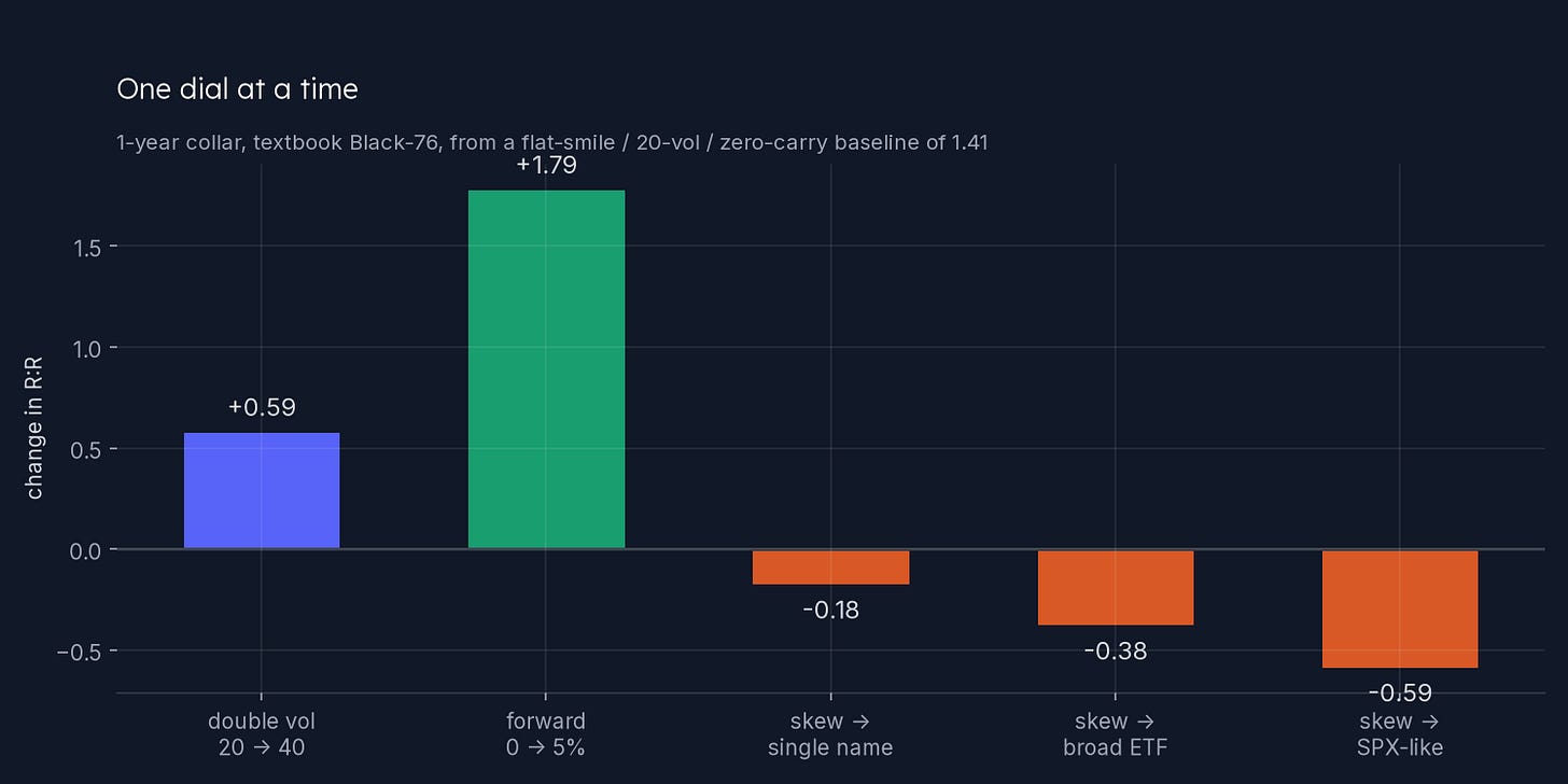
Observations

1) The forward is the big one by a distance. Going from zero carry to 5% nearly doubles the R:R. Intuitively this makes sense. If the options are priced against a stock price that’s 5% higher than the spot price, the puts are going to be much cheaper and the calls are going to cost much more. Think of it this way…the collar is comprised of a short .25d call and long a -.25d put, so it has -.50 delta in total. If we raise the spot price 5%, the collar premium falls by 2.5% of the spot price!

2) Doubling volatility also gives you better odds. That’s because the OTM call gets expensive faster than OTM put because increasing the vol, all else equal, on a lognormally distributed stock price extends the right tail while the downside is still floored at zero. You can review this concept in both Lessons From The .50 Delta Option and Finding Vol Convexity.

3) Equity-style skew works against you, ranging from a small drag on a typical single stock to something comparable to the whole vol effect on an index. This is mechanical and quite predictable. We are literally pumping up the IV of the puts and removing IV from the calls, making the collar more expensive. SPX-style skew has the same magnitude impact relative to the baseline as doubling vol (although the sign is flipped, as the collar gives you worse odds. It’s not cheap to hedge systematic risk!)

4) Tenor. What happens if we increase time to expiry from the 1-year baseline? We don’t need to model it because we know that increasing time is the same as increasing volatility. Variance is proportional to time, so volatility is proportional to √T. Doubling the vol is the same as quadrupling time.

That is the whole reason long-dated collars look better all else equal.

market prices

Let’s turn to option chains. These are based on median parameters across n tickers for each tenor based on EOD marks on 8/7/26:

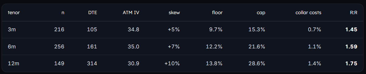
Skew steepens with tenor and the collar gets more expensive in cash, the R:R still improves, since the forwards and increased time is pulling harder than skew is pushing.

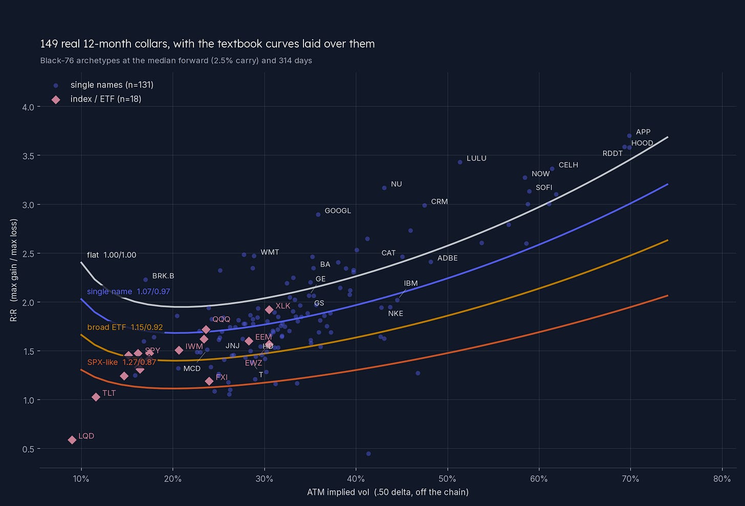
Laying the textbook curves over the risk-reward of real 1-year collars:

Time series view

The cross-section is one day but here are 1-year collars through time on five liquid ETFs, with their parameters plotted underneath it.

• Solid line is the ratio (left axis)
• Dotted lines are the ATM vols and the normalized skew (right axis)

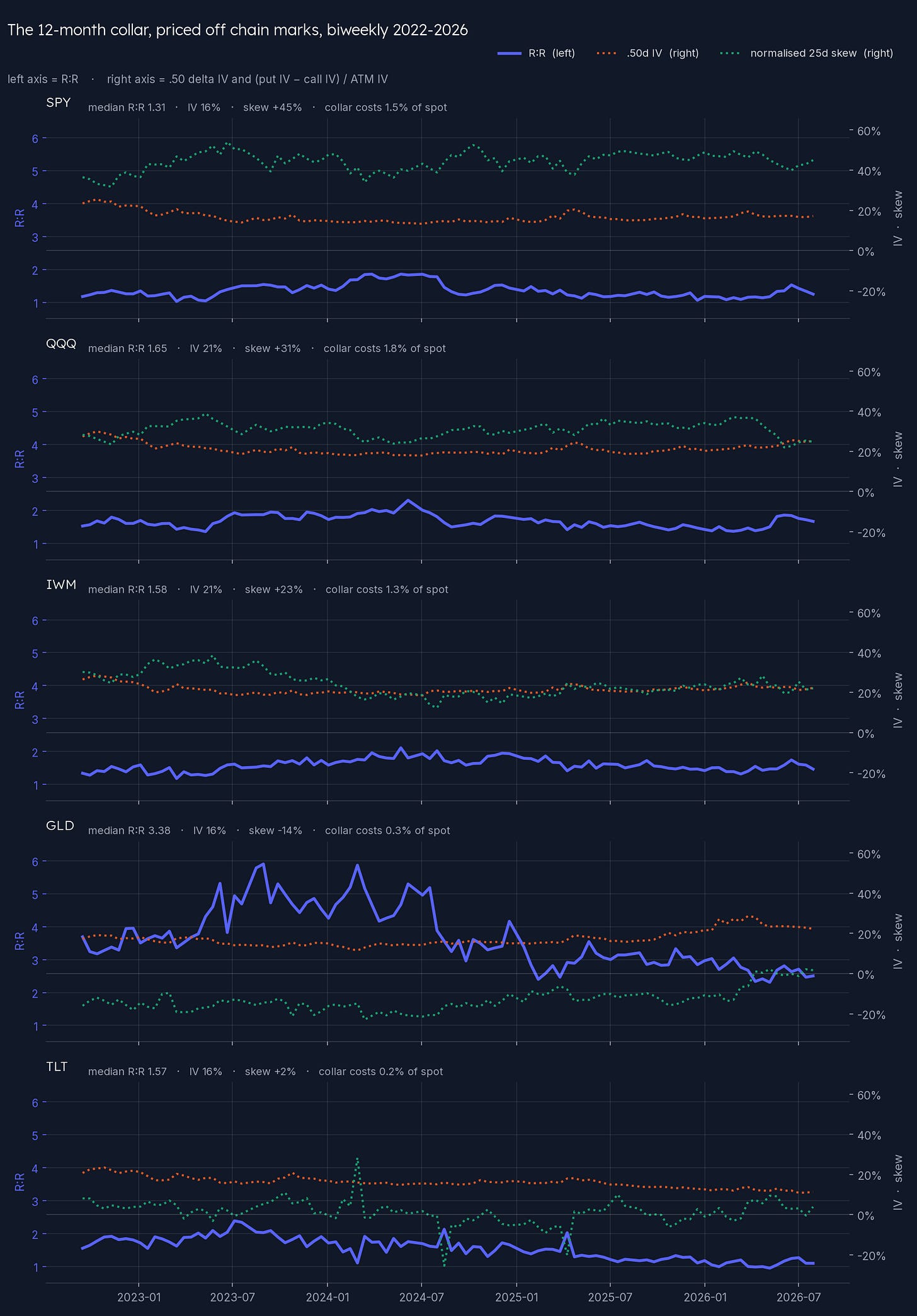
Eyeballing the charts, what pops out to me is how much more volatile skew is than the vol itself is for 1-year options and that variation is moving the R:R.

You also see how gold’s risk premium sits on the call side. It is the thing people panic into, so the fear bid lands on upside, and the .25 delta call trades over the .25 delta put, which sets up extremely attractive R:R for investors that want to hedge gold downside. Of course, there’s not much demand for that unless maybe you’re a miner, and even then, their IR and management teams probably know their investors want unhedged exposure to the metal. The other way you could see this is the cost to hedge gold upside is more lop-sided than the cost to hedge SPY downside!

Takeaways

1. Compare collars of the same maturity, or don’t compare them. R:R rises with tenor mechanically. In our cross sections they were 1.45 at three months, 1.59 at six, 1.75 at twelve, across the same names on the same day. A twelve-month collar that looks better than a three-month one has told you nothing. This is why the Collars Workflow tool keys off a chosen maturity rather than showing you whatever expiry happens to look good.

2. Vol moves the ratio, but not as much as you’d think in practice. Doubling volatility from 20 to 40 takes R:R from 1.41 to 2.00. That’s a big jump but required doubling the vol. Twelve-month vols don’t do that. SPY’s twelve-month ATM vol spent the last four years between 13.3% and 25.5%, standard deviation under 3 vol points. The move you’ll actually see are worth about .1 in the ratio or 1.4 vs 1.5 R:R.

3. A sense of proportion around skew and the R:R. Dialing from flat to index-like skew moved the R:R from 1.4 to 1.9 in our 20 vol archtype. Same magnitude as doubling the vol!

4. The forward is the biggest lever. Zero to 5% carry takes R:R from 1.41 to 3.20. The forward is directly dependent on the RFR. When interest rates are high, collars are going to look very attractive.

5. Tenor scales like vol but as a square root power function but linearly with the forward effect. A constant vol propogates the R:R at a rate of √T while carry scales linearly with T. Double the tenor and the vol dimension grows 1.41×, the carry dimension 2×. Both effects make long-dated collars look attractive.

6. A high ratio is a description, not a grade. 1.7 on a typical single name at a year is common but would be a gift in SPY and posion in GLD. Suggests comparing R:R across similar names or asset types.

Appendix

What is priced

Own the stock, buy the .25 delta put, sell the .25 delta call, roll the net cost into your basis. Exactly what the Collars Workflow shows.

• basis = spot + (put mid − call mid)
• max loss = basis − put strike
• max gain = call strike − basis · R:R = max gain / max loss
• Floor is 1 − Kput/spot
• Cap is Kcall/spot − 1
• The collar’s price is shown as a percent of spot.

Where the numbers come from

• Moontower end-of-day option chains and Greeks
• The .50 delta call’s IV is the ATM reference.
• Normalized skew is (put IV − call IV) / ATM IV, so a 1.3 put against a 0.9 call reads +40%
• The only modeled numbers in the post are the textbook Black-76 dials and archetype curves, which are labelled as such and use no market data.
• Legs are the listed strike whose own delta is nearest 0.25, rejected if it misses by more than 0.08.
• Nearest listed expiry to target, inside a DTE window. 3m [70,110], 6m [152,212], 12m [305,425].
• Actual DTE medians are 105, 161 and 314 so closer to 3.5 months, 5.5 months, and 11 months

Why the archetype curves dip into a smile shape

R:R is a ratio of a cap to a floor, so it inherits every pathology of dividing by a small number. At low vol the floor collapses toward zero so the ratio increases quickly.