

Back in May, I shared a Jane Street-style interview question I found online.
Flip a fair coin 100 times. Call the number of heads H and the number of tails T. What’s E[H × T]?
I multiplied the expected number of heads by the expected number of tails to get 2,500. I flubbed the answer because, while the flips are independent, the totals aren’t. Every additional head means one fewer tail.
There’s a missing covariance term in the way I set up the problem.
If you’re interested in the solution and all of its logic, review turning a Jane Street interview question blunder to a lesson.
In Socrates 2026, I talk about a project where I use LLM’s as patient math tutors to fill in basic gaps in my knowledge that the coin question’s solution alerted me to. Over the past few months, I’ve been spending some free time deriving useful forms of variance and covariance identities. I explained to Claude that my primary intent was to learn about these topics in the context of portfolio construction and that I did not want it to give me answers, but it could use leading questions to direct me.
But after every break, maybe I’d go 2 or 3 weeks without working on it, I’d need to back up, rederive something again to get loosened up, and move up the next rung. One step back, two steps forward as I ratcheted my way through the list. Once I felt I “owned” the concept, I’d have Claude append it to a growing cheat sheet.
I’ve published it here for you as a reference:
📓 variance and covariance cheat sheet
I think it’s both a neat consolidation and progression, but anyone can prompt AI to make them something like that. Of course that’s not the same as building up to it with AI in the manner I described, but the merit of that exercise is up to your own priorities which I’d expect are mostly different than mine. (I don’t consider this work. It’s a fun leisure activity that I get excited to do once I eat my obligatory vegetables).
The paywalled part of this post will get to application, but I want to talk about learning a bit more before we get there. By tediously deriving the identities on pen and paper, the literal motion of the strokes ingrains the abstract patterns. In an increasingly on-demand info landscape, it’s dangerous to forget that it’s difficult, maybe impossible, to shortcut understanding. It’s easy to parrot and getting easier, which means in the “zig where others zag” recipe for the scarce, specific knowledge you want demands seeking terrain that you’d be excited to cross, touch and feel where others would simply fly over and take a picture. A picture they’ll probably never look at again. They only flew over the terrain in the first place because someone said it was cool, and this FOMO-fueled podcast addict thought they could learn it in 45 minutes at 2x speed.
[The moment you realize there are infinite things our addict could survey in this hasty way, he should wonder how his info diet became what it was instead of the billion things it didn’t but could have been. It’s an uncomfortable question because it creates FOMO about the things you should have FOMO about instead of things you currently have FOMO about. Part of the joy of working through tedious things is how it focuses you and turns the volume down on the FOMO. Gee, it’s almost like exercising options is more fun than collecting them.]
Why deriving the identities on the cheat sheet is satisfying
It’s satisfying to start from the basic definition of variance as the mean of squared deviations and convert that to the expression of variance that is used to derive various versions for finance purposes.
Var(X) = Mean of squared deviation
is equal to
Expectation of random variable squared MINUS average of random variable squared
In notation:
Var(X) = E[(X − μ)2] = E[X2] − (E[X])2
I like to use actual numerals to understand these variable-heavy expressions. This graphic shows how these expressions tie out with an example.
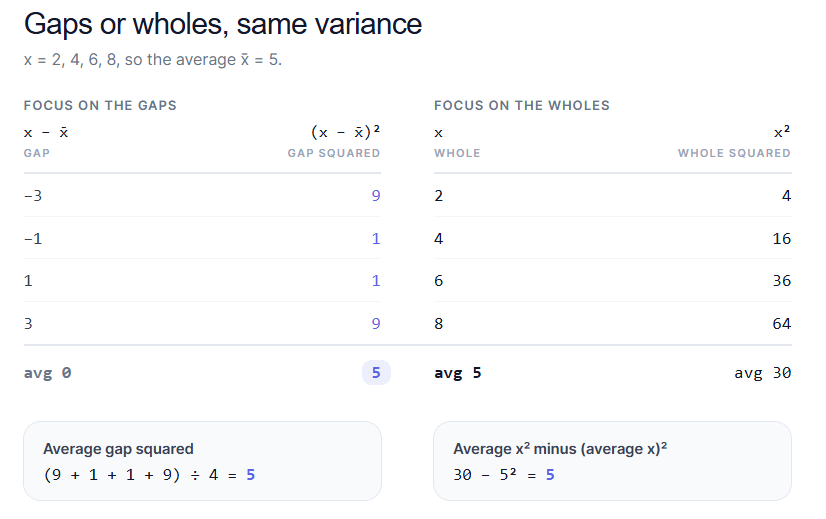
This singular expression: Var(X)= E[X2] − (E[X])2 is the starting template to derive many useful formulas algebraically.
Here I used it to derive the variance for a 3-asset portfolio. In the red boxes are my little reminders for the base expression (upper right) and how to expand a generic trinomial (bottom right).
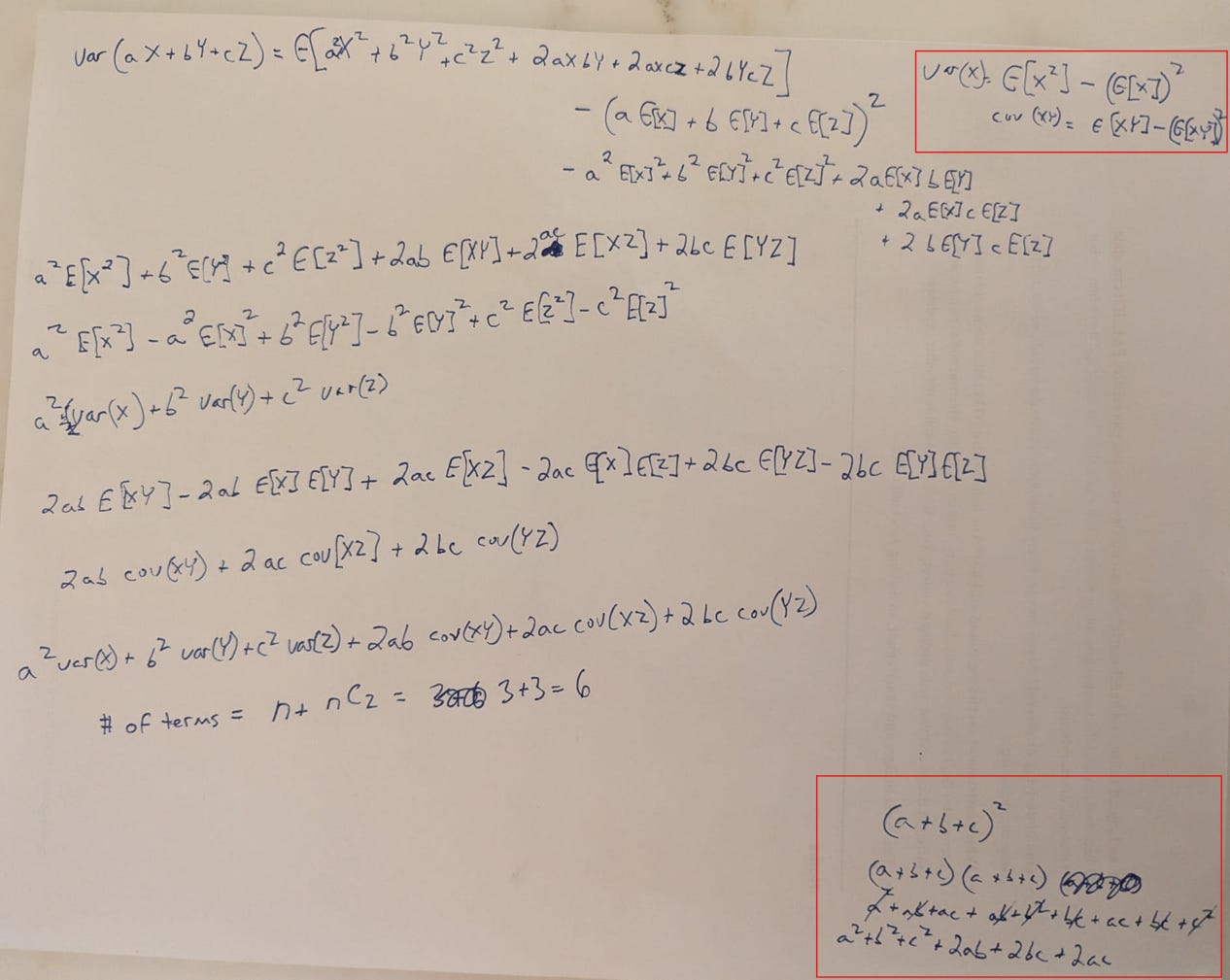
In working through this, you get used to the patterns from the algebra, noticing how many cross terms there will be. I figured once I did this for the trinomial, I’d see where each term lives in a covariance matrix for this relatively simple case of 6 total terms:
- 3 variances, one for each stock (which you can also think of as the covariance of each stock with itself or the diagonal on the correlation matrix
- plus C(3,2) covariances, or the number of pairs you get from 3 stocks.
6 terms means lots of algebra, and since the number of terms grows in proportion to n2, you will never do this again, but feel like you have the right to use the compressed matrix math.
If you work through the derivations starting from the basic variance expression, you start to see the reason for portfolio construction tenets that you have heard but not verified.
For example:
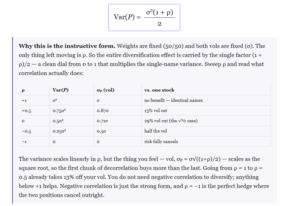
How correlation changes portfolio risk. Split your money equally between two assets with the same volatility. At a correlation of 1, you get no reduction in volatility. At zero, variance is cut in half. At −1, the fluctuations cancel completely. You don’t need negative correlation to get a diversification benefit.
Where inverse-variance weighting comes from. For two uncorrelated assets, the minimum-variance portfolio weights each in proportion to the inverse of its variance. An asset with twice the volatility gets one-quarter as much weight. Allow covariance and the optimal weights change.
What the covariance matrix is counting. Each asset contributes its own weighted variance while each pair contributes a covariance term. The matrix organizes those terms. The familiar factor of two in the two-asset formula comes from counting both mirrored entries: the covariance of A with B and of B with A. On the diagonal, an asset’s covariance with itself is simply its variance.
Var(aX + bY) = a2 Var(X) + b2 Var(Y) + 2ab · Cov(X, Y)
The derivations mostly repeat the same steps: start with the definition, expand, take expectations, and collect terms. Working through them makes it easier to see which assumptions a shortcut needs.
Read the entire variance and covariance cheat sheet →
Let’s put the math to work
We’re going to get practical.
It’s strange to think that a “crappy” asset can be worth buying, but for an asset to be crappy it means investors buy it! If it had little demand, its performance would be stronger, and it wouldn’t seem crappy.
So a crappy asset feels like something that is actually too well bid. To understand how that can happen, especially for assets we wouldn’t see as sexy or particularly coveted, we get to apply the math in the cheat sheet.
We start with a useful question:
Suppose an asset has a lower Sharpe ratio than your portfolio. How much lower can it be and still improve the portfolio?
You can probably guess that the answer has something to do with the correlation to what you already own.
We’ll examine ETF returns for typical portfolios both with and without commodities, across a generation of performance, and see how they contribute to risk and return and test a guess on what variable sharply divides how additive (or not) they have been.
How much worse can it be?
Sharpe measures average return above cash per unit of volatility. A higher standalone Sharpe means an asset delivered more excess return for the variability you endured owning it alone.
But you’re considering adding it to a portfolio.
For a small allocation, the hurdle is:
The new asset’s Sharpe must exceed its correlation with your portfolio multiplied by your portfolio’s Sharpe.
Suppose your portfolio has a Sharpe of 0.50. An asset with a correlation of 0.20 only needs a Sharpe above 0.10 to improve it at the margin.
That asset can have a much worse standalone Sharpe and still help.
It’s the same point as the SUN/RAIN example in You Don’t See The Whole Picture: an asset that pays when the rest of your portfolio doesn’t is worth more to you than to someone holding it alone. It means whoever owns the offsetting risk should be the best bid for it. [This is a sneakily important point that predicts that a good diversifier will be overpriced on a standalone basis.]
Here’s the same comparison at a few correlations:
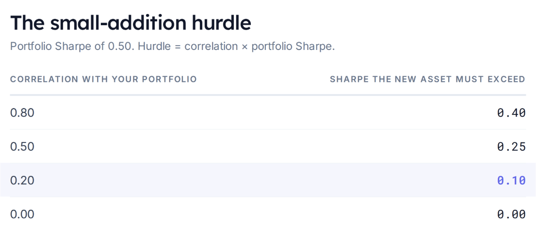
Even though the lower correlation lowers the return hurdle, it doesn’t eliminate it. (Appendix A derives the rule.)
The phrase “small allocation” matters. This tells you whether the first addition helps. It doesn’t tell you how much to own.
How “much” to add?
Consider a hypothetical portfolio earning 12% with 20% volatility. Cash earns 2%, so its Sharpe is 0.50. A prospective diversifier earns 5% with 15% volatility, giving it a Sharpe of 0.20. Its correlation is 0.20.
Here’s what happens as we replace the original portfolio with the diversifier:
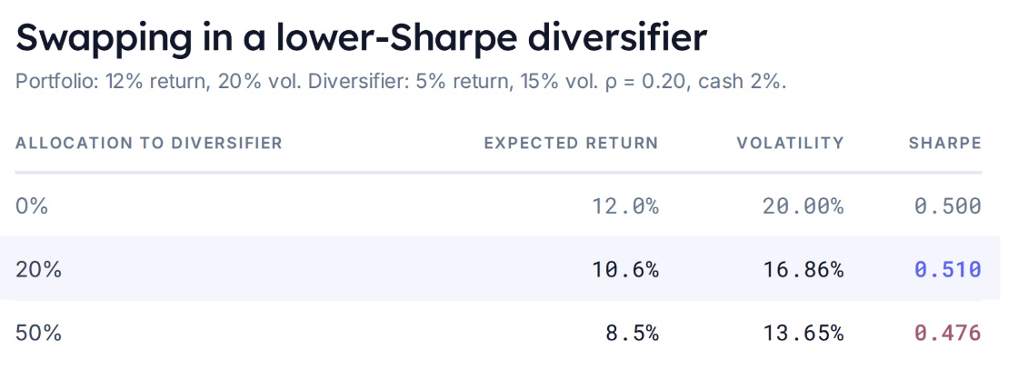
At 20%, excess return falls, but because volatility falls proportionally more, Sharpe improves, but at 50%, we’ve given up too much return for the additional reduction in volatility.
Appendix B walks through this example and gives the exact hurdle for a specified weight.
The key takeaway:
Identifying something worth adding and deciding how much to add are separate calculations.
Let’s apply this idea to actual investments
I fetched twenty years of monthly ETF returns, August 2006 through July 2026. Returns include dividend and distribution adjustments, and Sharpe uses monthly returns above a Treasury bill benchmark. Details in Appendix C.
Start with a portfolio that’s all SPY. Build six alternatives, each one 80% SPY plus 20% of a single candidate, rebalanced to those weights at every month-end. The 7 different portfolios:
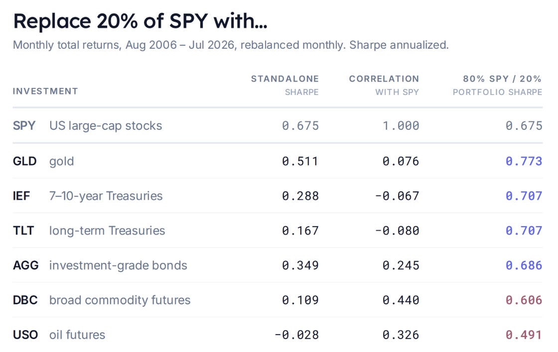
One objection before the results. Nobody knew gold’s twenty-year correlation with SPY in 2006. These are full-sample numbers, computed once across all 240 months, and they use information that wasn’t available while the portfolio was being held.
But that’s fine, because this isn’t a strategy. It’s a description. We are trying to isolate what correlation did to a portfolio, which requires seeing the whole sample.
Notice how correlation isn’t an input to the sizing either. Every candidate gets the same 20%, regardless of its correlation, because we are not yet addressing “how much?”.
Gold and treasuries improved the portfolio’s Sharpe despite considerably lower standalone Sharpes.
DBC and USO did not.
For DBC, the small-addition hurdle was approximately 0.44 times SPY’s 0.675 Sharpe, or 0.297. DBC’s realized Sharpe was only 0.109. Its correlation was below one, but its return relative to volatility wasn’t sufficient to improve SPY’s Sharpe.
USO also failed the hurdle. Not shocking. After all, these are returns on futures funds. USO’s performance is comprised of M1 returns + the return of rolling from M1 to M2. Since WTI has spent much of its history in contango (an upward-sloping curve kind of like VIX) the rolls have dragged down performance. In other words, the funds are not as straightforward as just owning spot oil because of the storage cost embedded in the rolls. Gold, on the other hand, has minimal storage costs and itself can be repo’d to offset some of its time value of money carry costs.
So far, the exercise gives us examples on both sides: lower-Sharpe assets that improved the portfolio and lower-Sharpe assets that didn’t.
But the commodity results raise another question.
When did commodities help?
My intuition was that commodities might be useful when bonds struggle. Inflation can be bad for nominal bonds while commodity prices rise.
[This intuition is messy but valid as demonstrated by the Inflation Replicator.]
Now the first test I tried was to examine the years in which AGG’s returns landed in their bottom quartile. Among the nineteen complete calendar years in the sample, that produced five: 2013, 2015, 2018, 2021, and 2022.
From here onward, the comparison is a 60% SPY / 40% AGG portfolio versus 60% SPY / 30% AGG / 10% commodities. The commodity allocation comes out of bonds.
DBC improved portfolio returns in only two of those five years. USO helped in three.
2021 and 2022 fit the intuition. But 2015 brought large commodity losses. Selecting weak bond years had grouped together episodes in which commodities behaved very differently.
“Bonds did badly” didn’t feel precise enough to test the inflation idea.
A more direct question is: did commodities improve the portfolio during months when inflation expectations rose?
We need an observable measure of inflation expectations.
Enter Treasury “breakevens”. The breakeven is the nominal Treasury yield minus the inflation-protected Treasury yield. It measures market-implied inflation compensation.
[Because TIPs are much smaller markets and less liquid than nominals, plus, well, the entire weight of financial theory’s distinction between risk-neutral and real-world probabilities, this measure of inflation expectation is imperfect. Surrendering to streetlight effects, we will presume the imperfection is more than made up by the observability of the measure.]
We’ll use monthly changes in FRED’s ten-year breakeven series. A rising-breakeven month is one in which the final available observation exceeds the previous month’s final observation. No additional requirement that stocks or bonds fall. (Appendix C has the series details.)
There were 122 such months in our twenty-year sample.
What happened to portfolio Sharpe?
First, compare average returns and volatility across those 122 months. Then divide mean excess return by its standard deviation to get the conditional Sharpe.
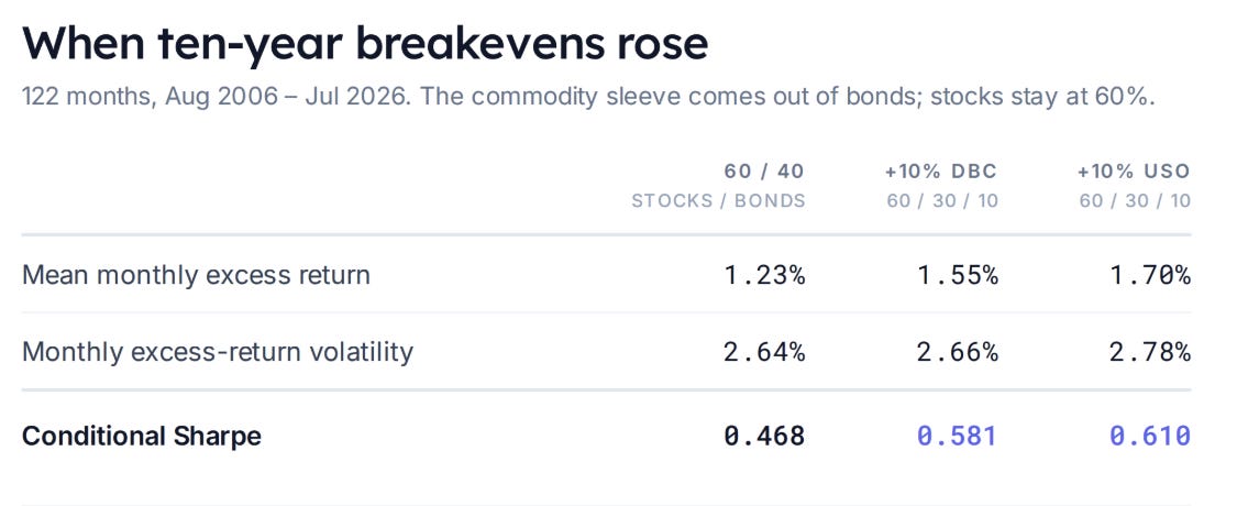
Both commodity allocations improved realized return per unit of volatility.
DBC barely changed portfolio volatility. USO increased it somewhat more. In both cases, the additional excess return more than compensated for the additional variability.
For comparison, here’s the same calculation when ten-year breakevens fell:
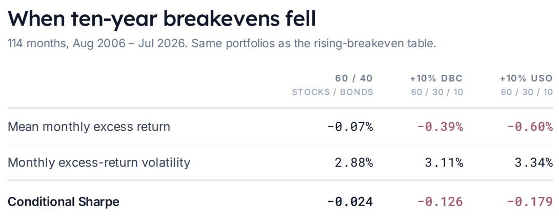
When breakevens fell, adding commodities reduced average excess return and increased volatility. The direction of the result reversed.
How much confidence should we put in it?
The improvement in rising-breakeven months was positive in both ten-year halves of the sample. It also held when I used five-year rather than ten-year breakevens. (Both checks are in Appendix D.)
To assess sampling uncertainty, I resampled the history in blocks, keeping each month’s breakeven change and portfolio returns together. In each resampled history, I selected rising-breakeven months and recalculated the difference in Sharpe.
Bootstrap
This resampling technique asks what else this history could plausibly have looked like. It cut the twenty years into blocks of consecutive months, restitched them into a new twenty-year history, and redid the calculation 20,000 times. The middle 95% of those answers is the interval. Blocks rather than single months because breakevens and returns arrive in runs, and shuffling month by month would erase that (Appendix D has the details and the limits).
The estimated Sharpe improvement was 0.114 for DBC and 0.143 for USO. The corresponding 95% bootstrap intervals were entirely positive: 0.074 to 0.153 for DBC, and 0.071 to 0.227 for USO. Changing the block length didn’t change the conclusion.
So what does this mean for the allocation?
Across all 240 months, adding commodities to the 60/40 portfolio reduced its Sharpe. (The full-period Sharpes are in Appendix C.) During rising-breakeven months, both commodity allocations improved it. During falling-breakeven months, both worsened it.
It’s important to recognize that nothing here is predictive. It is coincident, in that it shows how DBC and USO improved portfolios when inflation expectations increased. For those of us building portfolios to capture risk premiums instead of playing Nostrodamus, this is valuable insight into which assets help when inflation risks take center stage. It’s not surprising since commodities are both direct and indirect drivers of inflation, but seeing it in return data is affirming.
Kris, what’s the upshot?
The result alone doesn’t establish that commodities deserve a particular permanent weight. Commodities, at least as proxied by USO and DBC, hurt the portfolio across the full sample. They kicked in when you wanted and expected them to help, but you “paid” for that with all the underperforming months.
Theoretically, this makes sense. Inflation is both hard to hedge and destructive, as it incinerates the value of “stored work” in the form of savings. Assets that perform well when inflation gets scary should be overpriced.
For the investor or allocator, perhaps this means:
- tilting towards commodities if you believe that inflation will be a larger issue in the next 20 years vs the last generation.
- finding commodity exposures that have less drag
- ignoring commodities but also nominal bonds, giving you less inflation risk in your portfolio to start with
Wrapping up
The goal of this post was to animate the math of return variances, something you could have learned in stats class, to see how it informs portfolio construction, which is the final boss of risk management since it’s ultimately about dosing.
"Crappy" is a verdict on an asset held alone, but nothing is held alone. The thing that looks worst by itself is the thing someone else needs, which is why it never looks cheap. The ramifications of this are important and we’ll build on that in a later post.
For now, you can see the appendix for nitty-gritty. I included references back to the cheat sheet for things we applied in the post.
Run the study yourself
The companion code downloads the source data and runs the calculations in a Google Colab notebook. Choose between two modes:
- Reproduce the post: use August 2006–July 2026, with the same ETFs, portfolio weights, monthly rebalancing and statistical methods used here.
- Refresh the study: keep the same starting date and methodology, and extend the analysis through the latest complete month available across all required series.
Both modes retrieve ETF adjusted prices, FRED breakevens and the monthly cash benchmark directly from their sources, then generate the portfolio comparisons and bootstrap results. The repository contains the retrieval and analysis code; you download the data when you run it.
Feel free to fork it and add your own flair!
Open the notebook in Colab · View the code on GitHub
Appendix: calculations, assumptions and sources
A. Deriving the small-addition Sharpe hurdle
Let A be the existing portfolio and B the prospective addition. All means, volatilities and correlations below refer to excess returns over the same cash benchmark, measured over the same horizon. Write their expected excess returns, volatilities and correlation as:

Put a fraction w in B and keep 1 − w in A. The portfolio’s mean and variance are:

This is the cheat sheet’s weighted-sum workhorse, Var(aX + bY), with a = 1 − w and b = w and the cross term written through the correlation definition.
The sheet stops at portfolio variance; differentiating the Sharpe is the new step.
At w = 0:

Apply the quotient rule to the portfolio Sharpe:
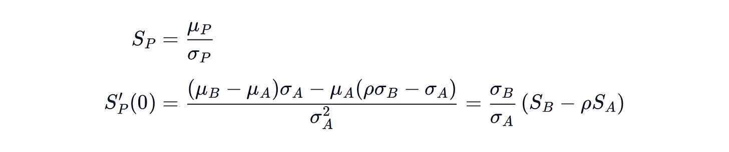
The volatility ratio is positive. The first small addition improves Sharpe when:

B. The worked example and finite-weight hurdle
Toy assumptions: A earns 12% with 20% volatility; B earns 5% with 15% volatility; cash earns a constant 2%; correlation is 0.20. Expected returns are arithmetic means, not CAGRs.
At 80% A / 20% B:
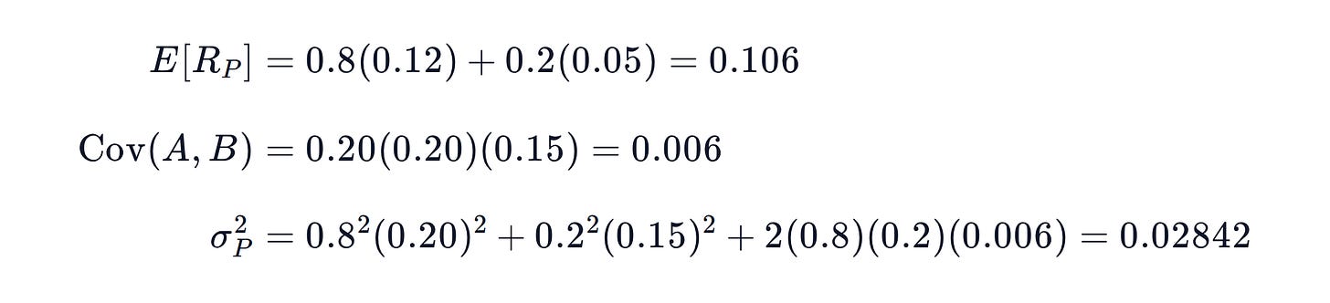
Thus volatility is 16.8582% and Sharpe is:

For a specified weight 0 < w < 1, define:

Factoring (1 − w) times A’s volatility out of portfolio volatility gives:

Provided portfolio volatility is nonzero, rearranging the condition that portfolio Sharpe exceeds A’s Sharpe gives the exact hurdle:

As the allocation approaches zero, the multiplier approaches ρ. At a finite allocation, relative volatility and weight also matter.
C. Data and portfolio construction
All empirical results are DERIVED. The common window is August 2006–July 2026: 240 monthly returns, using July 2006 month-end prices as the starting observation. Data were retrieved September 21, 2026. The end date is the latest common month supported by the retrieved risk-free series. No missing observations were filled or pre-inception histories spliced.
ETF returns. Daily Yahoo Finance adjusted closes, sampled on the final available trading day of each month. Monthly return is the ratio of successive adjusted prices minus one. This is a distribution-reinvested market-price return proxy, adjusted for splits. Distributions are not added again. Fund expenses are reflected; investor taxes, trading costs and rebalancing costs are excluded.
Historical-price pages: SPY, GLD, IEF, TLT, AGG, DBC and USO. The retrieval code will identify the source endpoints and retain the actual price dates used in each run. USO’s sponsor describes the futures-based fund; its history should not be interpreted as spot-oil ownership.
Cash benchmark. Monthly RF returns from the Kenneth French Data Library, July 2026 vintage. Source percentage values are divided by 100. Download.
Breakevens. FRED T10YIE and T5YIE. Use the last nonmissing daily observation each month and subtract the previous month’s endpoint. Rates are quoted in percent; multiplying the difference by 100 expresses it in basis points.
Rebalancing. Each portfolio is reset to its stated weights monthly. Monthly portfolio return is the weighted sum of that month’s ETF returns. The first comparison uses 80% SPY / 20% candidate; the commodity condition study uses 60% SPY / 40% AGG versus 60% SPY / 30% AGG / 10% DBC or USO.
Sharpe. Subtract monthly RF from each portfolio return, average the selected excess returns, and divide by their sample standard deviation using n − 1. The first full-history ETF table multiplies this ratio by √12, the conventional annualization that does not adjust for serial correlation. The conditional tables leave the ratio monthly because they describe selected, nonconsecutive months. Do not compare their levels directly with the annualized table.
The conditional volatility is variability across selected monthly excess returns. It is not intramonth volatility or a drawdown measure. Neither the positive-breakeven sample nor its Sharpe represents an allocation rule that knew the month’s condition in advance.
For reference, all-240-month, unannualized Sharpes for the 60/40, DBC and USO portfolios are 0.201, 0.189 and 0.168, respectively.
Initial weak-bond-year screen. Calendar-year returns are compounded from monthly returns, including monthly rebalancing for portfolios. The nineteen complete years are 2007–2025. The bottom-quartile cutoff selects five years, or 26.3% of the observations; partial 2006 and 2026 are excluded. Improvement means higher annual portfolio return, not higher annual Sharpe.
D. Stability and uncertainty
Monthly conditional Sharpes during rising breakevens:
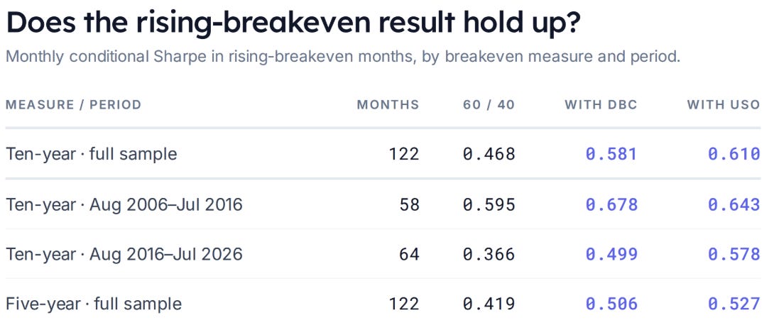
The five- and ten-year measures happen to select the same number of rising months, but not identical months. The split-sample results are stability checks, not independent out-of-sample validation.
What the bootstrap does. We have one observed history. To gauge how much its estimated Sharpe difference might vary with the sample, draw six-month blocks from the full chronological dataset and stitch them into another 240-month history. Keep breakevens, cash returns and all portfolio returns paired. Reapply the rising/falling condition and recalculate the Sharpe differences. Repeat 20,000 times.
Blocks preserve some persistence in conditions and returns. We use a circular moving-block bootstrap, so blocks may wrap from the end of the dataset to its beginning. The 95% percentile interval spans the 2.5th to 97.5th percentiles of the resampled Sharpe differences.
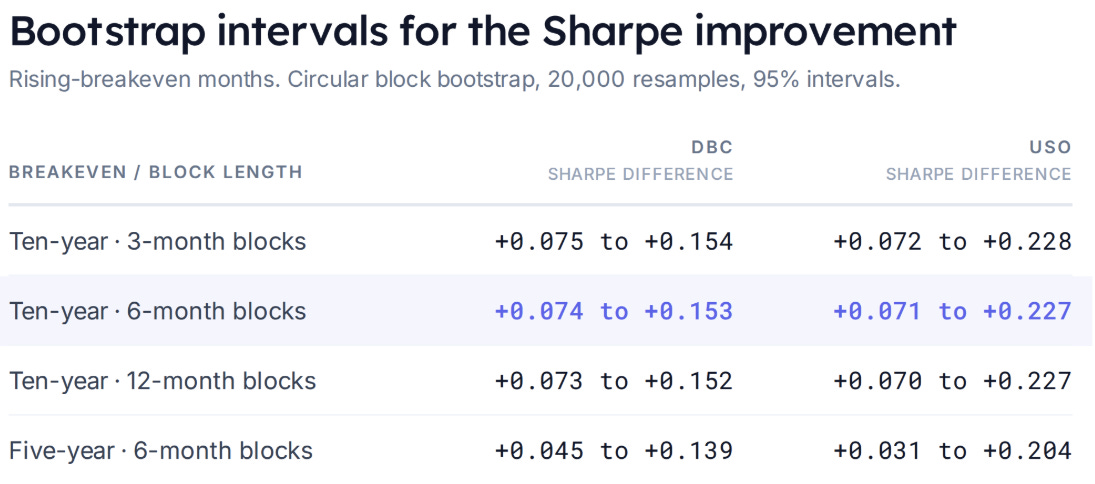
Six months is the primary block length; three and twelve months are sensitivity checks, not an optimized choice.
This was an exploratory analysis. Long-range dependence and structural changes may not be captured by the resampling method. It does not create independent historical evidence or establish causality. Oil can influence breakevens, both can respond to growth news, and breakevens include risk and liquidity compensation. The study answers an ex-post conditional portfolio question.