betting on direction with short-dated spreads

I’ve published several posts in the past month about option collars.

• collar shopping
• the risk-reward of option collars
• additional thoughts on the risk-reward of option collars

Most of what I’ve written leans on an artifact of option pricing namely that the further out in time you go, the more call premium there is to work with. I started talking about this in May’s high implied vol can work for or against you. High IV makes calls grow faster in value than puts, which can make it more attractive for hedgers to finance downside.

The quirk comes from option pricing conventions that assume a stock moves in percentages. Percentages compound, which makes the model symmetric in logs and lopsided in dollars.

The whole asymmetry:

ln(1.05) = +4.879%
ln(0.95) = −5.129%

To sit the same log distance from 100 as a move up to 105, the stock has to fall to 95.24, not 95.00, but this is not symmetrical to investors who think in percents. If you want to dwell on this further, bookmark understanding log returns and using log returns and volatility to normalize strike distances. The net effect, and what we care about, is that continuous compounding creates a wedge between expected mean and median returns, commonly referred to as “volatility drag” (or “variance drain” as it was taught to me in trader training 25+ years ago). The wedge is a function of variance and time.

Gap between mean and median: exp(−σ²T/2)

Consider a $100 stock at 45 vol. Assume 0% expected growth (option models usually use the risk-free rate in no-arbitrage pricing frameworks, but our assumption doesn’t affect the point).

The 1-year median outcome = 100*exp(-.5*.45²) = $90.37

Nearly 10% below the forward!

Note that if the stock’s expected mean return were +10%, your median outcome would effectively cancel out. This sounds dissonant, so some perspective is in order.

The way to interpret the wedge between mean and median is that a small proportion of wildly positive stock moves contribute to that 10% expected return, but a significant portion of the time, the stock’s volatility causes it to ratchet lower, dragging down the median return. High-vol assets rely on lower-probability up moves to boost their expectancy, because the high vol itself is a source of downward pressure when you compound up 5%, then down 5% over and over.

In a sense, high volatility is a picture of positive skewness (option surfaces can correct for this, of course, by discounting OTM calls and boosting OTM puts, but the basic lognormal distribution bounded at zero is naturally positively skewed). Long-dated collars inherit this natural skewness, which boosts OTM calls faster than OTM puts.

…But today we are going to talk about trading short-dated verticals (collars are a type of vertical). And we can talk about them like a sharp saloon gambler because all of these weird compounding artifacts melt away in the short-term.

You can see this if we compute the median discount as we did above on our $100 stock for different terms:

1 year median stock price $90.37 —> $9.63 discount

1 month —> $.83 discount

1 week —> $.19 discount

2 days —> $.06 discount

Again, this assumes 0 expected arithmetic return. If we assume a risk-free rate or more for expected stock return, we are in the world of return symmetry, which coincides with our intuition.

What’s the probability the stock goes up tomorrow? 50/50 bruh.

What’s more likely, up 2% or down 2%? Same bruh.

When it comes to the short-term, no stochastic option calculus. Our focus today is going to be on sizing up vertical spreads as bettors. This requires pricing the spread and sizing trades (which you should be able to do in your head with little effort once you step through a few of the worked examples). This is a big post in that if you chow down both the meat and side dishes, your entire understanding of options will experience a major upgrade. There’s also a nugget which acts as a test to how much your understanding of options is really “getting it” or if you are still trapped in “calls and puts are just levered stock trades” land.

What’s the spread worth?

The rule for a short-dated spread:

If the stock is sitting halfway between the two strikes, the spread is worth half the distance between them.

My definition of short-dated is arbitrary, but let’s say less than 5 calendar DTE. So no longer than a Friday expiry if it’s Monday morning.

If the stock is 27.50, the 25/30 call spread is worth $2.50. This is the price expression of “It’s 50/50 bruh”.

So what about option skew?

Option skew refers to how OTM options trade at a different implied vols than the at-the-moneys. In equity indices, OTM puts generally trade at a premium IV to the ATM and OTM calls trade at a discount. Individual equities often exhibit the same behavior, but the skew is less steep. Meanwhile, some equities, those that exhibit “spot up, vol up” momentum, can have inverted skews where OTM call IV > OTM put IV. Inverted skew is also fairly common in commodities and precious metals.

That’s all nice background knowledge, but it doesn’t have a significant influence on short-term option pricing by the time we get into betting space.

Scenario

Stock = 27.50

DTE = 5

25 strike put @ 40% IV = .9 cents

25 strike put @ 42% IV = 1.3 cents

30 strike call @ 40% IV = 1.7 cents

30 strike call @ 38% IV = 1.2 cents

With “flat” vols between the strikes, the call is worth .8 cents more than the put (this is a collar with the call premium to the put). That’s mild lognormality showing up in a 40 vol name (something like TSLA).

A traditional skew makes the collar worth about zero, flipping the structure’s value by less than a penny. The option vegas (their sensitivity to IV) is small with only 5 DTE to the skew has “nothing to push on”.

The short-dated collar is the key to the vertical spread

I started talking about the call spread as our representative of vertical spreads and then switched to the collar to demonstrate the minimal impact of skew. But unless you are dealing with 2 OTM options, when you price a vertical you should do it by looking at the collar, then converting it to a call spread.

Let’s see why.

An in-the-money option has two parts:

• Intrinsic value: the distance between the strike and the stock. This is the value of the option if it expired right now.
• Extrinsic value: the time value of the contract. This extra value represents “possibility”. This is part of the option that is influenced by changes in implied volatility, since time and volatility both represent possibility.

Here’s a handy bit to understand:

For a given strike, the extrinsic value of the ITM option IS value of the OTM option!*

This is from the TSLA chain for a short-dated option when the stock was $347.98

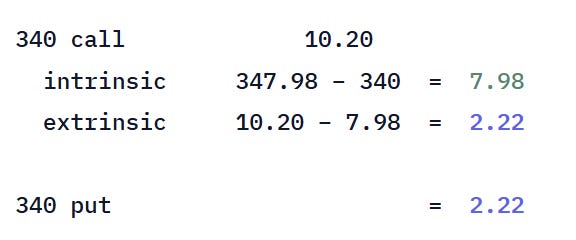
The algebra generalizes the fact that the 340 call is two things stapled together: stock exposure from 340, and a 340 put.

Let’s build a 340/355 call spread vertical but substitute:

F − K1 is simply intrinsic value.

But we want to rearrange this into the form for turning the collar, which we will easily observe from an option chain, to get the market’s fair price of the call spread.

If you prefer a visual, this graphic shows what option position you’d need at each strike to create a synthetic stock position, call spread, or collar, respectively. Notice how owning a collar (long put/short call) + a synthetic stock position gives you a long call spread!

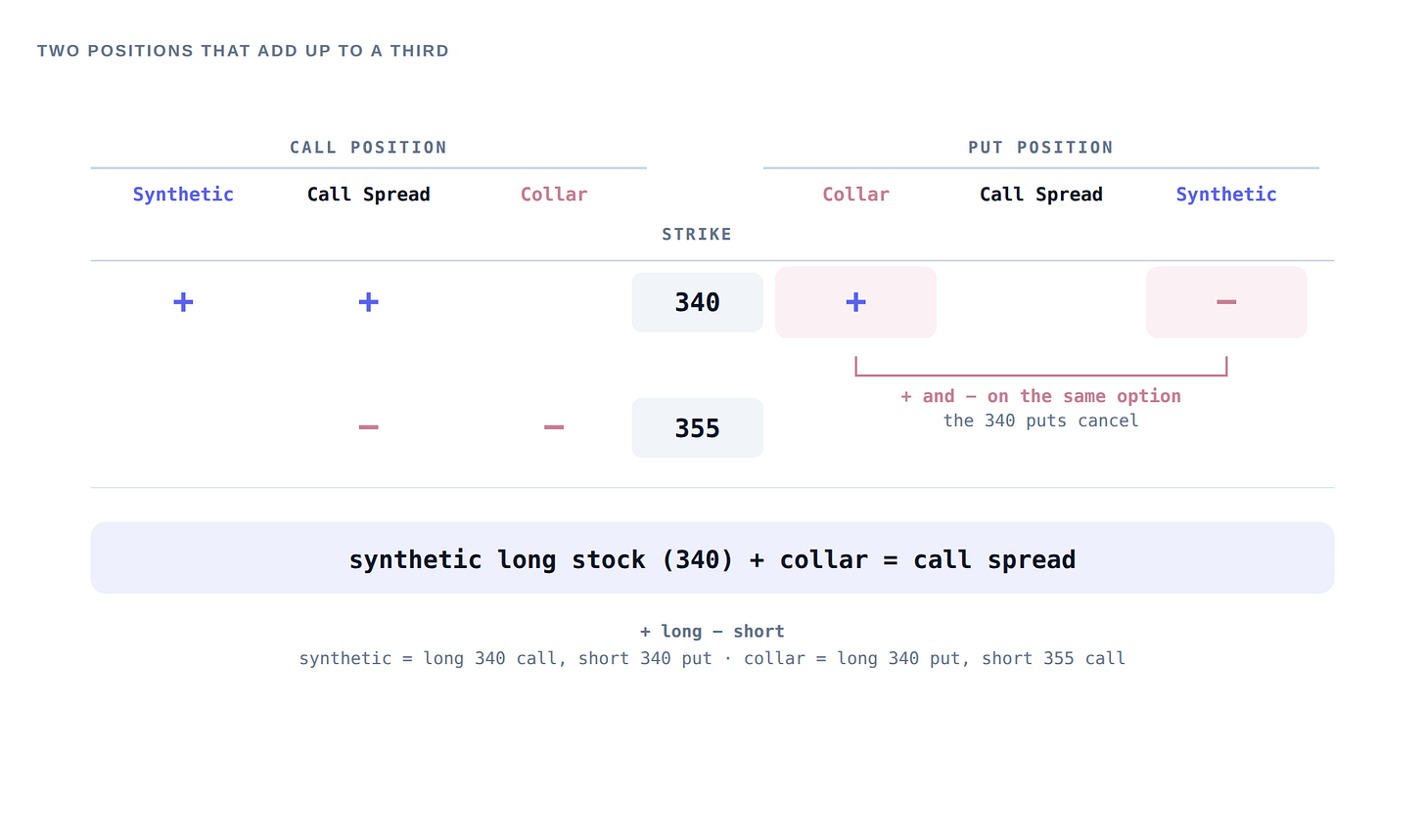
You can prove equivalence by inventing prices for the options and the stock and comparing p/l at expiration under different stock prices for the call spread versus the package of a synthetic + collar.

You can also see that holding the stock constant, if the 340 put goes up in value (ie IV is increasing), the call spread is also gaining value! This might seem counterintuitive, but it’s the same idea. The put skew increasing can be interpreted as the stock’s left tail is longer, but for that to be true with the stock in the same place, then the probability of the stock rising must be increasing to counterbalance. A call spread increasing in value with the stock in the same place is a binary bet on whether the stock will be higher or lower but not a bet on the magnitude (ie HOW much higher or lower). So it is perfectly consistent that the put and call spread increase in value together (again holding the stock price constant).

If this is confusing, it’s because you see options as directional instruments, not distributional surfaces. You are still stuck in “call means up” and “put means down” when, in fact, calls and puts are the same.

It is this graduated understanding that lets you price the 340/355 call spread better because you never touch the wide ITM option.

Let’s practice.

Pricing the 340/355 call spread

TSLA, Wednesday, August 26th 2026, options expiring that Friday. Two days out, no earnings that week.

At 10:03 ET in the morning, the stock was $347.87.

Take the 340/355 call spread so the stock is near the midpoint.

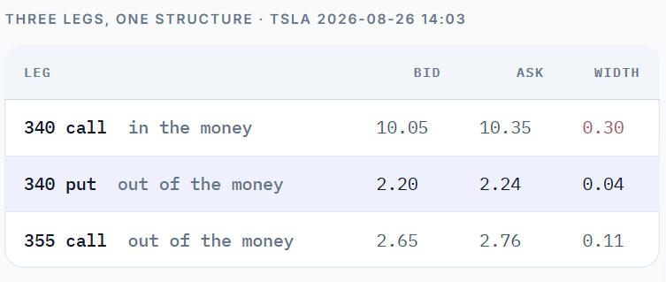
The 340 call mid is $10.20, and we’ll say the 355 call is $2.70, yielding a mid-market call spread price of $7.50.

But let’s price the call spread from the tighter put market.

The 340 put mid is $2.22. We add that to the intrinsic value of $7.87 to get a call value of $10.09.

$10.09 - $2.70 = $7.39

To purchase that call spread “synthetically” for the $7.39 price, you need to buy the stock for $347.87 and the 340/355 collar for a CREDIT of $.48.

Do you see how you end up with a net debit of $347.39, but $340 of that is basically the stock value of the $340 strike? You have paid only $7.39 above $340, which is the same as if you bought the actual call spread for $7.39. In both cases, you are protected below $340 (in the synthetic case, you own the 340 put), and capped after $355 (you are short the 355 call either way).

The key is that the market price of the 340/355 call spread is obscured because the 340 call market is 30 cents wide! But your knowledge of synthetics allows you to price it off the puts (and the market makers’ knowledge of synthetics plus speed allows them to arb between real and synthetic prices all day).

The difference in width between ITM and OTM options is a regularity:

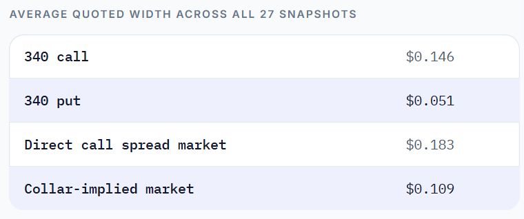
The call spread value implied by the collar is almost 50% tighter.

From market value to taking risk

Thus far we’ve made the claim that a near-dated vertical spread should be priced like a bar bet. The spread should be worth half the distance between the strikes if the stock is at the midpoint. This claim is reasonable in light of how little skew and assumptions of lognormality affect short-dated options.

From there, we used knowledge of put-call parity to allow us to see market pricing based on the most liquid legs.

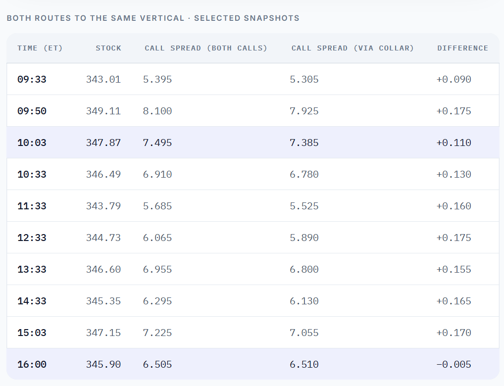
A long call spread (either an actual call spread or the synthetic one) is a bullish directional trade with the downside capped to the premium and the upside capped to the strike distance minus the premium. If you buy a $ 15-wide call spread for $7 you risk $7 to make $8.

But it’s worth remembering that this proposition represents the extremes and “at expiry”. In the meantime, the call spread has positive delta and will gain value with the stock and vice versa.

We can see that in the table of snapshots above, but here’s another view:

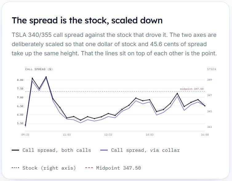
While the synthetic call spread has a tighter market, that doesn’t change the fact that it’s the same type of risk. The actual call spread and its synthetic version track each other all day (separated by a financing wedge deriving from the fact that the synthetic call spread is discounted because it requires financing a long stock position for a couple days).

But instead of a time series, let’s view the spread value vs the stock price as a scatterplot.

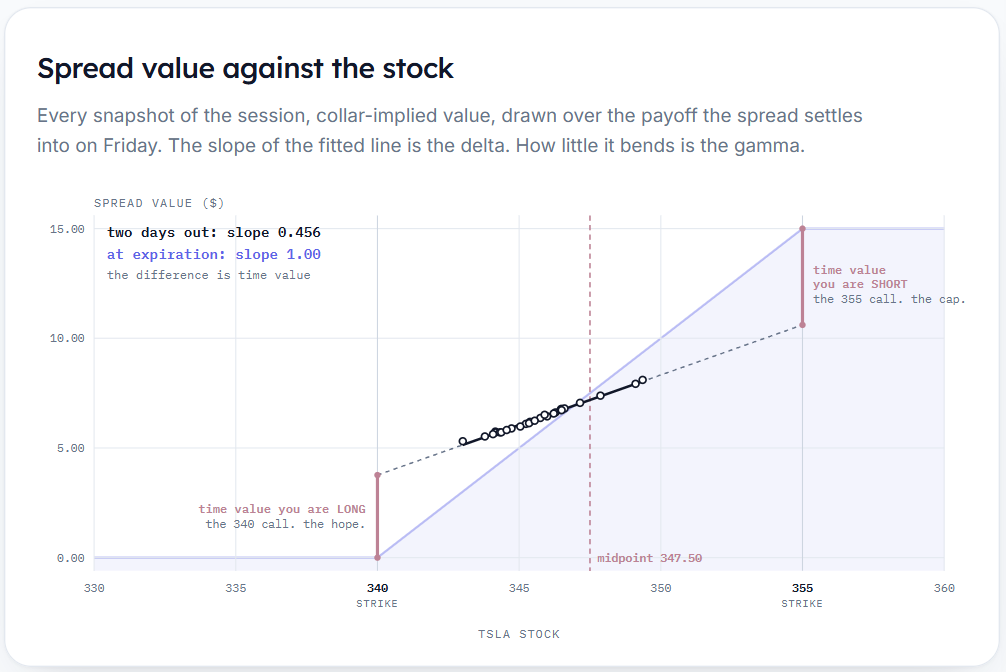
Things to notice:

• If the Y-axis is call spread value and the X-axis is stock price, then the slope is…delta! The spread delta is about .45.
• The purple line behind the dot is what the spread is worth at expiration. It’s the classic hockey stick diagram of a call spread. Inside the strikes, that line has a slope of exactly 1.00, because on Friday afternoon a dollar of stock is a dollar of spread and there’s no time left for anything else to happen.
• The live quotes trace a much shallower path (the .45 delta) through the same space.
• The straightness of the line reveals how little gamma there is in the spread. The delta is relatively constant over various stock prices. A position with real gamma would bend this scatter into a curve.

At 340, the spread expires worthless. But if the stock drops to 340 today, the spread isn’t worthless. Its value will be dominated by the time value in the 340 call you own (and offset modestly by whatever remaining optionality you are short in the now-far-OTM 355 call).

At 355, the spread is worth the full fifteen at expiration, but it would trade below that today even if the stock leaped to 355 or even 357. The shortfall is time value in the 355 call you’re short.

Discrete bets

To be complete about risk, I thought it was important to show the above charts so you understand the call spread does have continuous values before expiration, even though we tend to speak of them more in terms of their expiration payouts.

But let’s go back to thinking of call spreads as discrete or binary bets on where the underlying stock will be at expiry.

Divide a call spread by its width, and you get the market’s odds that the stock finishes above the spread’s midpoint.

Examples of various spreads and the risk-neutral probabilities they imply:

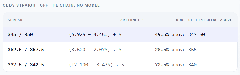
Going back to our friend the 340/355 call spread, we can look at the prices the way you might look at prediction market prices, as probabilities:

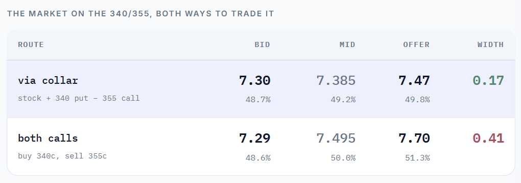
Lifting the direct offer, you need to be right about the stock expiring above the midpoint 51.3% of the time to break even.

I can’t tell you how to predict the future (presumably have a model against which to compare to the bogeys that I’m teaching you to infer from the market). But let’s say your homework leads you to believe the market prices are over- or underestimating the probability of certain price moves…how do we size them?

Sizing discrete bets

Most of my trading had a continuous market-making feel to it. Your portfolio is a soup of positions from being counterparty to flows. A mix of risk management and biases informed my targets for position greeks like vega, gamma, and theta.

For siloed wagers, Kelly is a well-established framework for sizing risk is the loss is bounded and payoffs discrete. The vertical spread ideas qualify for that approach because you put up or receive premium, with a well-defined gain or loss.

The Kelly Criterion succinctly:

Kelly is the bet size, as a fraction of bankroll, that maximizes the long-run compounded growth rate of your wealth. It’s a mathematical solution to bet size that doesn’t seek to maximize expected profit per trial, but the size that optimally balances compounding rate and survival.

We will use this formulation of Kelly:

A few simple examples:

Fair coin

p =50%

q= 50%

b =1 (ie even money, for a $1 bet you either lose a $1 or make a $1 profit)

f* = 50% - 50% / 1 = 0 → bet nothing, zero edge

Coin biased in your favor

p =60%

q= 40%

b =1 (ie even money, for a $1 bet you either lose a $1 or make a $1 profit)

f* = 60% - 40% / 1 = 0.20 → bet 20% of your bankroll

Roll a 6 on a die

p =1/6

q= 5/6

b =8 (for a $1 bet, you either lose a $1 or make an $8 profit)

f* = 1/6 - (5/6) / 8

f* =8/48 - 5/48 = 3/48 → bet 6.25% of your bankroll

If f* is 0 or negative, you have no edge, so not betting is prescribed

Worked example on call spreads

Assume you pay $7.47

risk = 7.47
win = 15.00 − 7.47 = 7.53
odds b = 7.53 / 7.47 = 1.008

Even money, near enough, which is what you’d expect for a spread whose midpoint is sitting on the stock.

Set f* to zero and you get the break-even view:

p = 1/(1+b) = 49.8%.

That is exactly 7.47 / 15, the price-over-width number from the odds table.

Now say you think there’s a 70% chance TSLA closes above $347.50 on Friday:

f* = 0.70 − 0.30/1.008
= 0.70 − 0.298
= 0.402

Forty percent of the bankroll at full Kelly. Half is 20%, quarter is 10%.

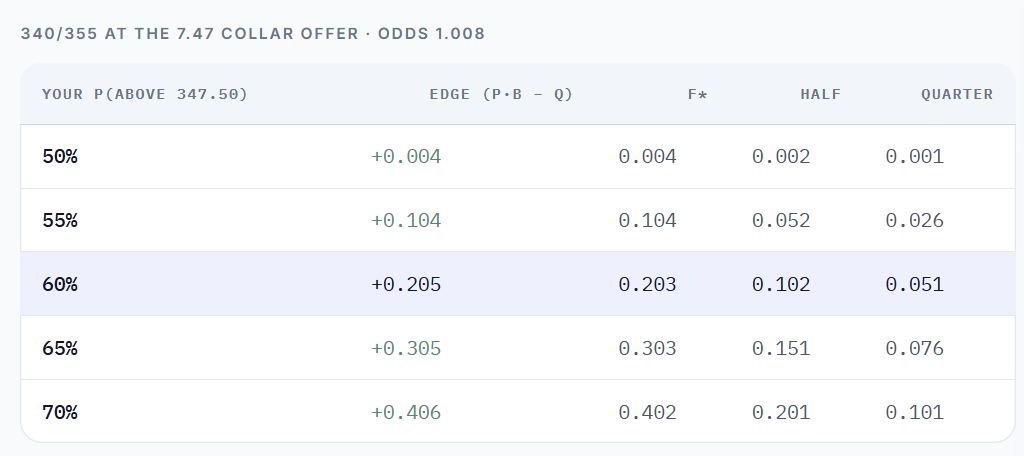
A note on execution

At that 60% view, paying the collar offer justifies 20.3% of bankroll. Paying the direct offer at 7.70 drops the odds to 0.948 and justifies only 17.8%

Better execution doesn’t just save you money on the trade; it lets you trade bigger on all ideas! This explains how trading firms can compound on tiny edges.

Betting on $355

Let’s do another example where you are more of an underdog.

Say you want to bet the stock finishes above $355 by Friday. The structure that expresses that is the 352.5/357.5 call spread, midpoint $355.

The stock is at $347.87, so both legs are already out of the money. There’s no in-the-money option in the trade, which means no need to use the collar to pinpoint the fair market pricing.

352.5 call 3.45 / 3.55 (10 cents wide)
357.5 call 2.03 / 2.12 ( 9 cents wide)

buy the spread: 3.55 − 2.03 = 1.52
sell the spread: 3.45 − 2.12 = 1.33
mid: 1.425

Let’s say the spread trades mid, 1.425. Divide by the width:

1.425 / 5 = 28.5% → the chain’s probability of finishing above 355.

Paying the offer moves your break-even to 1.52 / 5 = 30.4%, so the offer costs you about two points of probability.

Now the odds:

risk = 1.52
win = 5.00 − 1.52 = 3.48
odds b = 3.48 / 1.52 = 2.289

Better than 2 to 1, because you’re buying something that probably doesn’t happen.

Say you think it’s 45% to expire greater than $355:

f* = 0.45 − 0.55/2.289
= 0.45 − 0.240
= 0.210 → full Kelly is 21% of bankroll

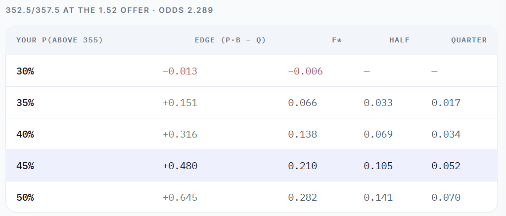
From the table, we see the 30% row is negative, which is the formula telling you don’t bet.

Notice that a 45% view against a 28.5% market is a bigger “disagreement” than the 70% view in the first example, and it still sizes smaller. When you’re getting 2.29 to 1, a loss costs you less of the bankroll, but you also lose far more often. Kelly considers both.

What we learned

• The lognormal tilt is a compounding artifact, and compounding needs time. The positive skewness you harvest in the collar posts hasn’t had a chance to accumulate yet.
• Near-dated, the gambler’s intuition is the correct one. Stock sitting between two strikes, few days to go, no earnings…the vertical is worth about half the width. “50/50 bruh” is a good guess on what the math converges to.
• Price the vertical off the collar, not off the ITM call. The 340 call was 30 cents wide. The 340 put was 4. Use put/call parity to turn an OTM option into an ITM leg.
• Price divided by width is the market’s probability of finishing above the midpoint. The tighter the spread, the more reliable this approximation.
• This means you can invert a vertical spread into a probability to quantify your edge. The market gives you a p to compare with your own p.
• Kelly turns that disagreement into a size. f* = p − q/b. It’s built for discrete bets with a known payoff.
• Full Kelly is for psychos.