additional thoughts on the risk-reward of option collars

I know this is an off-cycle post but I just want to add a couple of important insights as a brief follow-up to last week’s the risk-reward of option collars.

As a reminder, that piece starts with a highly intuitive (ie what actual investors think about) measure of an option collar’s risk-reward and the aspects of the vol surface which push it up or down. The point is to marry the vol lens with the price lens people use to actually make an investing decision.

And for those of us who don’t want to think too hard when looking at pictures, I also include a section on chart craft.

Let’s roll…

A sense of proportion around skew and vol sensitivities

Originally, showed the effect of turning various dials one unit at a time to isolate the price impact on risk-reward.

For the vol dial: Doubling vol from 20 to 40 moved risk-reward from 1.41 to 2.00.

For the skew dial: Going from index skew to single-stock skew moved it about as far the other way.

By putting those dials side by side, I risked making you think these moves were equally likely or similar in magnitude. But a natural question would be “What if doubling volatility is a four-standard-deviation event and the skew move is a two?”

To make a fairer comparison, here’s the same analysis with everything measured against how much the vol and skew actually change.

Method for estimating sensitivity

• Four years of the twelve-month collar on SPY, QQQ, IWM, GLD and TLT
• Price each one at 20 vol with no carry, keeping only its own skew shape
• Shock it by its own history
• Re-price the collar
• Measure the change

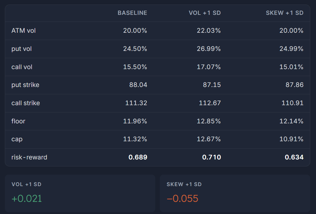
Observations

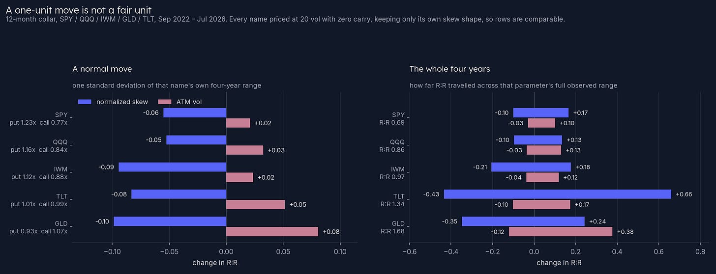
1) A normal move in skew has a larger impact than changes in IV

One standard deviation of twelve-month ATM vol runs 1.5 to 2.9 points. This represents vol-of-vol. Meanwhile, a 1 standard deviation change in normalized skew is 4.0 to 6.6 points depending on the name. Trace the changes through an option model and you see that the variation in vol is worth +0.02 to +0.08 of risk-reward while skew is worth −0.05 to −0.10.

• Skew is the bigger lever in all five names
• More vol helps a collar slightly, but more skew hurts it more.

2) Predictably, at the extremes, the risk-reward of a collar can move substantially, but it doesn’t in SPY

The right panel takes each parameter’s full four-year range rather than a typical move. Vol’s whole observed range is worth about a fifth of a turn on the equity ETFs. For example, SPY spans −0.03 to +0.10 across a vol history that ran 13.3% to 25.5%.

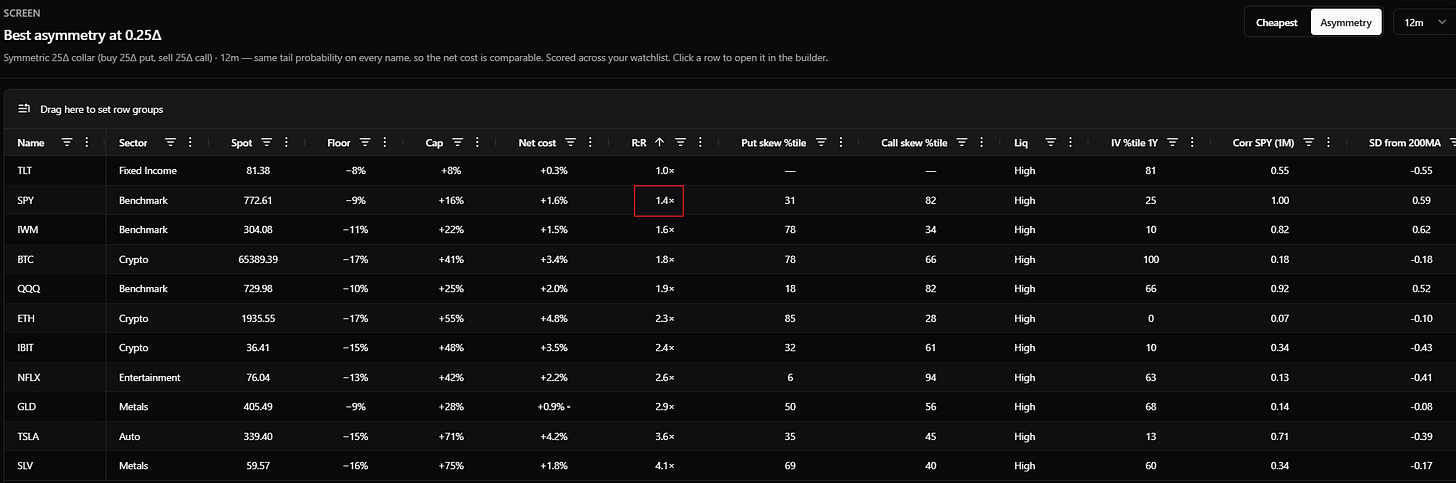
This is 8/17/26 and despite 1-year SPY puts being relatively low and calls being relatively high, the juice never gets worth the squeeze. The r:r is still roughly what it always is over the past several years.

That said, overall, skew has a wider sweep of value to influence r:r.

Calling back to our time series, IWM skew spans −0.21 to +0.18. And TLT, whose normalized skew crossed from −.25 to +.28 over the four years, spans a risk-reward range of −0.43 to +0.66, more than a full turn from one parameter, on a collar whose base case is 1.34.

3) How much does risk-reward move?

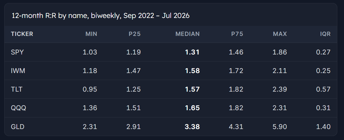
We already hinted at this, but SPY spends half its life inside a band a quarter of a turn wide. Equity indices in general don’t exhibit a lot of variation with respect to the risk-reward of collars compared to bonds and gold.

I’ll let you draw your own conclusions about what this means for diversification and also the conjoined ideas that:

1. Whether you should pay for active management depends on manager dispersion within an asset class (see the chart on Mauboussin page 29)
2. What makes something worth trading in the first place

Technique: Rotating 3 dimensions in one picture

A short aside on chart craft.

A scatterplot with a color channel carries three variables at once, which sacrifices some detail relative to a 3-dimensional chart but I think gains way more in readability.

Below are four years of the twelve-month collar on five liquid ETFs, with vol and skew as the axes and risk-reward as the color. Green is that ticker’s best quartile, orange its worst.

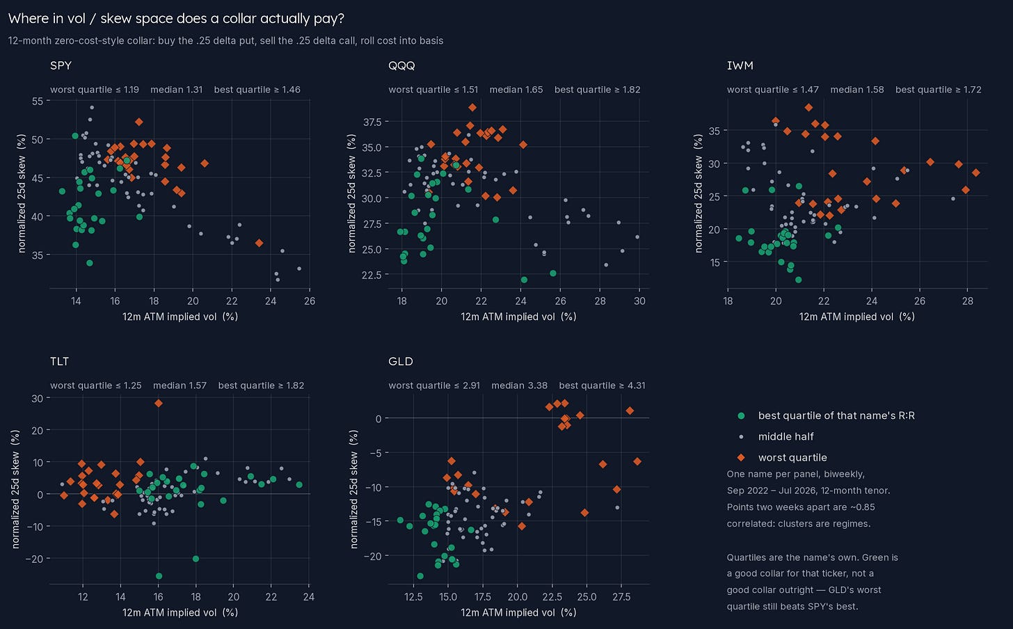
[It’s not the point of this post but I often say that skew flattens as vol increases and vice versa in SPY. It’s very clear in that chart. While we like to measure normalized skew percentiles, skew levels are not independent of IV, so it would be more insightful to condition skew percentiles on vol regimes if you’re trying to really pinpoint abnormal readings.]

Quartiles are specific to each name so green means an attractive risk-reward for the ticker but it hides the fact that GLD’s worst quartile of r:r is still better than SPY’s best quartile!

We need to rotate the axes and color code to see that.

Using the same data, we shift risk-reward to the vertical axis and skew becomes the color.

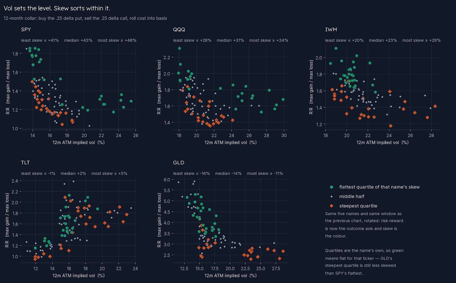
Now the question “what does skew do, holding vol roughly still” is just how far above the orange does the green sit at the same place on the x-axis. In four of five panels it floats clean above, everywhere along the range.