the option market's point spread (part 2)

In part 1, the option market's point spread, we introduced the idea of the VRP or volatility risk premium which sets the line on whether an option buyer or seller will win. Usually the sellers win but that statement is uselessly low res.

💡When we say “win” we mean even in expectancy terms. In frequency terms it’s even more true. From Straddles, Volatility, and Win Rates:

Expectancy and win rate are not the same. Remember that the most you can lose is 12% but since there is no upper bound on the stock, your win is theoretically infinite. So the expectancy of the straddle is balanced by the odds of it paying off. You should expect to lose more often than you win for your expectancy to be zero since your wins are larger than your losses.

So how often do you theoretically win?

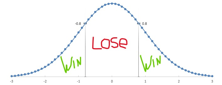
A fairly priced straddle quoted as percent of spot costs 80% of the volatility. We know that a 1-standard deviation range encompasses about 68% of a distribution. How about a .8 standard deviation range?

Fire up excel. NORMDIST(.8,0,1,True) for a cumulative distribution function. You get 78.8% which means 21.2% of the time the SPX goes up more than .8 standard deviations. Double that because there are 2 tails and voila…you win about 42% of the time.

So in Black-Scholes world, if you buy a straddle for correctly priced vol your expectancy is zero, but you expect to lose 58% of the time!

My teaser for this week’s post claimed:

[This week] we will go a bit deeper to appreciate how you can manipulate the inputs into VRPs to identify potential vol trades. I said VRP is the option market’s point spread.

Except for a tiny wrinkle.

There’s no single line.

The VRP computation (IV/RV) is just one measure of relative value. There’s no single point spread.

It’s easy to demonstrate this by casting doubt on the denominator. Here’s a thought exercise:

Stock ABC has a VRP of 10%.

Its IV is 17.6%

Its realized vol based on the last 20 days of daily log returns is 16%

📅16% annual vol is approx 1% per day…16%/sqrt(251)

17.6/16 = 1.10 - 1 = 10% VRP

…but

Now I tell you that the stock went up every single day by 1%.

💡If you compute the standard deviation the standard way by subtracting the sample mean (ie x̄) you’ll actually get a standard deviation of zero. If an asset has exhibited a steady trend this is obviously misleading since calling a stock that went up 1% per day for 20 days “zero vol” drains all semantic meaning from “vol”. The fix is easy…when you compute realized vol just don’t subtract the mean or use mean = 0 before squaring the individual returns. This caveat wasn’t the point of this exercise but if your antennae went up, fair play to you.

What’s the volatility of this stock?

Sampling daily returns we get 16%. But the stock is up 22% in 20 days.

We can annualize that point-to-point return:

22% * sqrt(251/20) ~ 78% realized vol

We can annualize the weekly (ie every 5 day returns):

5% * sqrt(251/5) ~ 35.4% realized vol

You get the picture.

What is the right vol for the option?!

16% seems way too cheap given what just happened.

So depending on what vol you pick your VRP ranges from 10% on the high end to 17.6/78 - 1 = -77% on the low end.

There’s not one point spread!

Realized vol is sensitive to your sampling periods. And I’m not even getting into super-fast updating vols (computing realized vols from tick data, a fun rabbit hole of its own).

On the desk, I was always on alert for highly divergent vol readings based on sampling periods.

[This is hardly a silver bullet. The implied vol on the hypothetical stock above is likely to be higher than 16%. The market’s not stupid.]

Honestly, I didn’t screen for those scenarios explicitly. I traded commodity options. The universe was relatively small so whenever I looked at realized vol numbers, which I did often, I had a feel for whether they made sense. If the realized vol (sampled daily) in gold is 12% but the metal is up 7% in 2 weeks I know the realized vol is misleading.

7% * √(52/2) ~ 36%

That’s like a 36-vol move. If near-dated options are trading at a 10% or even 20% VRP to 12% realized (or 13.2% to 14.4%) I’m out there accumulating a long gamma position.

I didn’t have a tool to necessarily flag these scenarios but if you trade a relatively short list of names all the time you build a mental history. I’d know which brokers were selling vol in the name, I might ask them where their customers are offering, or I might even go to brokers who were buying at cheaper vol levels before the move and see if they want to sell at the higher IVs and “take profits”.

[The game is a mix of what the cards are (examples include implied and realized vols) and human behavior —who has an axe to buy or sell and how do those axes change with the cards.]

The point is there’s a bunch of tacit knowledge that I don’t bother displaying on yet another monitor.

[There’s a wiseguys-trying-to-outdo-wiseguys snark about having lots of monitors. Like real Gs need nothing more than a laptop. You know something, being Warren Buffet or a VC is nice work if you can get it…but if you get the chance to visit the office of a market-making group you’re gonna see a LOT of screens. My set-up had 6 24s, a tablet for Cloud9, and windows into several virtual machines. What do you want me to say…professional trading is a video game. Put a price on 100k vega in comp, you have about as much time as it takes to move your eyes while chatting them up about last night’s World Series game.

I can see how a normal business person might think this is crazy. Lucky for them, most jobs are civilized. If you want to look down on the animals who need a wall of monitors you’re only soothing yourself — the feral don’t give a f what tool you use to convert time to cash.]

Using the data and background on VRP in last week’s post we can examine my tacit hunches more closely.

The goal of the post is to:

1. inspire seasoned traders to explore fresh inputs into pricing volatility
2. for novice traders, to have each of the building blocks in the exposition expand their frontier of knowledge a little further.

Ratio of realized vols sampled at different frequencies

In Risk Depends On The Resolution, we see that volatility depends on the sampling frequency. In general, more frequent sampling results in higher levels of measured volatility. This is a relevant observation for all investors not just option traders. It means that simply looking at an asset’s annual or even monthly returns smooths (if you are a long-term investor) or masks (if you run a strategy whose stakeholders are shorter-term oriented) the path. It’s a warm blanket for the patient and dragon for the churner. Whether the observation is reassuring or a warning depends on the context.

(I leave it to the reader to spot the asset management marketing departments who use this observation to flatter themselves by invoking it inappropriately).

For our purposes today we will measure 1-month realized volatility at 2 sampling frequencies:

• daily (day-over-day logreturns)
• weekly (5-day point-to-point logreturns)

Our monthly window will constitute 20 business days, therefore 1-month vol sampled:

daily means 20 returns or data points

weekly means 4 returns or data points

🗓️As a reminder we are using data from the past year (10/11/23 to 10/16/24).

Across our 43 names, the average ratio of volatility sampled weekly vs volatility sampled daily is 94%.

By example, that means a stock that realized 10% volatility using daily returns for the past month, would have realized 9.4% volatility if we sampled weekly instead.

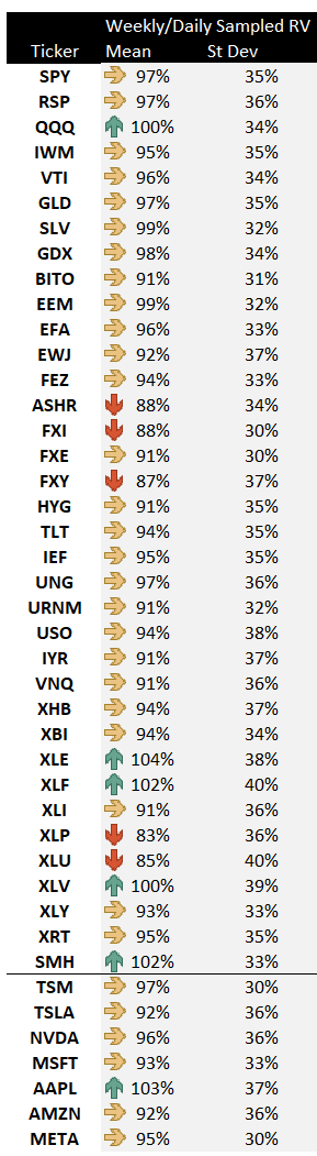
Only 5 names had a realized vol that was higher when sampled weekly instead of daily.

This is in keeping with the general empirical principle — volatility sampled less frequently tends to be lower.

However, there is tremendous variation in this ratio even if it averaged 94% over the full sample. The standard deviation of the ratio is a whopping 35% meaning 2/3 of the time the ratio was between:

• 59% — the daily sampled vol was 66% higher the weekly sampled vol!
• 129% — the weekly sampled vol was 29% higher than the daily sampled vol.

The lower measured vol effect from less frequent sampling holds generally, but it’s very noisy.

A word on trending vs mean-reversion

Going back to our introductory puzzle, if a stock goes up 1% per day for a month its vol, if we sample weekly, is much larger than if we simply annualize that typical daily volatility.

The ratio of vol sampled weekly / vol sampled daily is much greater 100%. This scenario corresponds to our colloquial understanding of the word “trend”. The stock “trended” higher. A quant might say the drift dominated the volatility. As far as I know, this ratio being > 1 is not an accepted definition of “trend”. But even if it is not formally defining, I suspect it’s a common characteristic of a market that is labeled “trending”. (I have a post in the queue that will unpack this further so we will put a pin it in for now.)

Regardless of how the wider quant community views trend, the ratio and its suggestion of trend is deeply relevant to option traders.

If the ratio is greater than 1, the long option holder will have wished “they let their gamma run” while the short option trader will have wished to hedge more frequently.

I suspect any option trader reading this will drink to that since the memory of how they hedged is inseparable from large p/l events, positive or negative.

Ya know what, let’s take a breath and acknowledge something…”ratio of realized vols sampled at different frequencies” is a miserable mouthful. Just take a moment to digest it. It refers to the same window of time, it’s just that the numerator (weekly sampling) is less frequent.

Another way to think of it: it takes longer to converge to a estimate of the volatility

If we computed volatility based on 10-year returns you’d die before you felt like you had a reasonable guess of the asset’s volatility. A long sampling period is a slow-moving measure of variation. Higher frequency sampling gets us to a reliable measure of volatility much faster.

While we’re at it, I have another simplification.

Sacrificing formality for ease of readability, let’s call the “ratio of realized vols sampled at different frequencies” the trend ratio. If the weekly sampled vol exceeds the daily sampled vol we are trending, if it’s lower there’s mean-reversion. (Again, not officially, and don’t tell the quant police or the publishers over at Wiley.)

From trend ratio to VRP

We typically measure VRP as the ratio of implied vol to realized vol sampled daily. But there’s no single VRP. We could make the denominator realized vol sampled weekly or any other interval.

Let’s consider a VRP using the weekly sampled vol.

If the weekly sampled vol is greater than the daily sampled vol (a trend ratio greater than 1), the VRP is algebraically pulled lower. Options appear cheaper.

We expect the options market to correct for this when the trend ratio is much greater than 1 by bidding the implied vol higher.

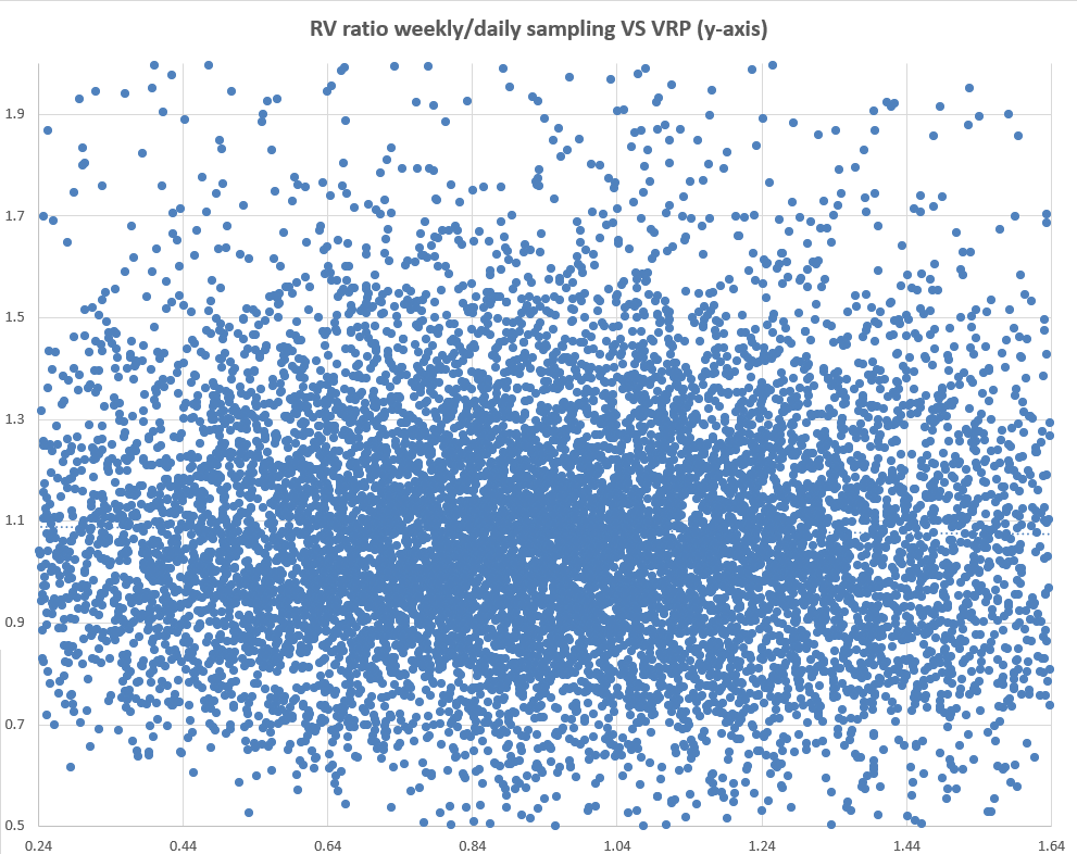
We expect that a trend ratio greater than 100% will coincide with elevated VRPs when the VRP is computed traditionally (ie with a daily sampled realized vol denominator).

Just looking at the bulk data across names (we limit the x-axis to 2 standard deviations on either side of mean of .94), there’s no relationship.

Let’s look by name.

This is a table of VRPs partitioned by trend ratio. The names that are mostly green have low VRPs and the red ones have had lots of volatility risk premium.

My hunch was that high trend ratios (where weekly sampled vol is much higher than daily sampled vol) would correspond to higher VRPs as the market understands that the traditional measure of realized vol is understating the variance. It’s like the variance is smuggled into a steady trend.

It’s a noisy table. At best maybe BITO and MSFT conform to my expectation. In fact, the broad indices (SPY, QQQ, IWM) and SPY sector indices (the “XL’s”) seem to have an even lower VRP when the trend ratio is highly positive. Considering that the market is up substantially from a year ago, the trend has been positive which tends to correspond with vol dampening option selling. This can push down the VRP via the numerator. Algebraically, it implies IV is well below realized vols that are computed using weekly sampling.

I did not expect this. My intuition is mostly tuned on commodities. I don’t see my hunch turned on its head there, but I don’t see a relationship either.

I have another idea. Since each name has its own mean VRP, let’s redo the table where each cell is a diff from the name’s own mean VRP.

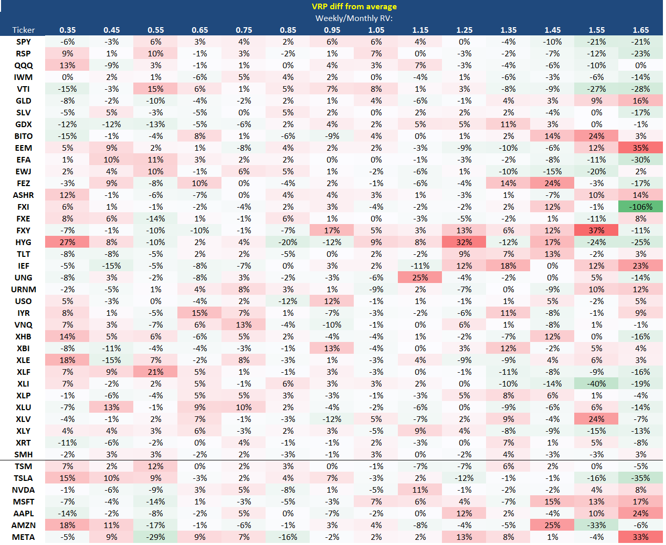
I’m getting the same feeling from this table especially in those broad indices. When the trend ratio has been much greater than 1, the VRP nosedives below its average. My suspicion is the vol is getting trashed on those steady “frog-in-the-pan” rallies.

Since the trend ratio is positive, the VRP based on the weekly sampled vol is even lower still!

This begs the question…were the options therefore cheap?

Trend ratios and lagged VRP

One way we can assess if the options were cheap is to look ahead in time to see if the realized VRP was less than 100%. In other words, did the realized vol that prevailed the subsequent month outperform the IV? We call this realized VRP a lagged VRP.

[Lagged VRP was a core topic in last week’s the option market's point spread]

This table once again partitions by trend ratio but now it displays the subsequent lagged VRP.

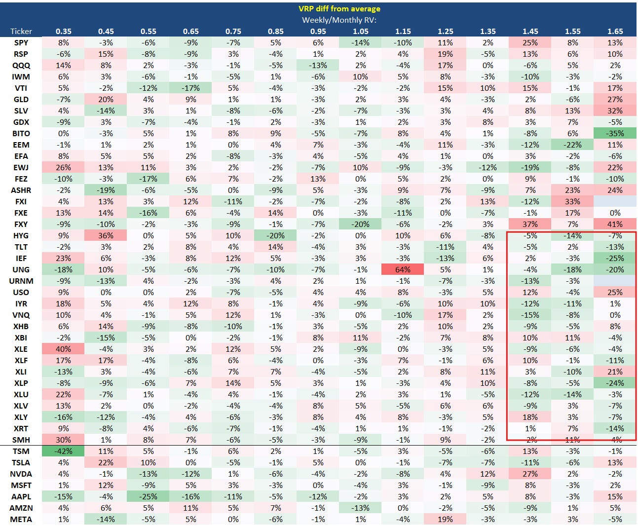
We do notice a preponderance of green amongst the XL sector indices suggesting the realized vols did in fact perform well vs the seemingly cheap IVs we spotted earlier.

But we did not see this hold for the broader indices. It also doesn’t mean that the IVs were absolutely cheap — after all, the lagged VRP’s on average are still higher than 100%…these options turned out to be fairly priced vs the subsequent realized vol.

Overall nothing stands out as blatantly interesting. At the same time, the non-finding, is also not a dead end. This exploration is incapable of being conclusive. It’s a year of data in 43 names with overlapping windows which means it’s not much data at all. Furthermore, the sample sizes in these individual cells is also small — sure when the XLU trend ratio was between 1.5 and 1.6 the options turned out to be cheap the following month but how often did that happen? That could be a sample size of 1. FXI and URNM never even experienced a trend ratio greater than 1.6.

Wrapping up

Like the last post, this was a demonstration of how to explore a vol idea. We started with the premise that realized vol measures can be a poor reflection of what an asset’s future volatility might be because its sensitive to the sampling period.

By choosing a different sampling period (which is what we effectively did by partitioning by trend ratio) we change the VRP which means changing how cheap or expensive the options appear. Then we see if our adjustments singled out vols that did in fact turn out to be mispriced.

There are so many parameters to play with. These were just a few from this post but you can imagine so many more:

• Realized vols from different sampling periods
• Different ways to compute realized vol (close-to-close vs range aware computations)
• Any number of implied vols you can choose from the surface.
• Asset classes, sectors, individual tickers

Personally, I start with ideas that make sense. If I measure realized volatility in 2 different ways and get vastly different numbers, it seems possible that the market might blend them incorrectly. Seems like a good place to look.

[💡General observation: The downside of an interpretable hypothesis, is you’ll probably have company. There are quant funds that generate signals they don’t even understand. The downside is when it goes wrong, it’s harder to troubleshoot. But at least nobody else is likely to find the edge while it persists.

In any case, that style of trading sounds like alien hunting. I am incapable of putting myself into the mind of alien to understand what it might do so it’s not a sport I’d think to play.]